staggered
Table of contents
Notes
- Based on: Roth and Sant’Anna 2023
-
Program version (if available): version 0.7.1 24Sep2024
- Last checked: 7 Jul 2026
Installation
ssc install staggered, replace
Take a look at the help file:
help staggered
Test the command
Please make sure that you generate the shared setup data using the setup block given here
Let’s try the basic staggered command:
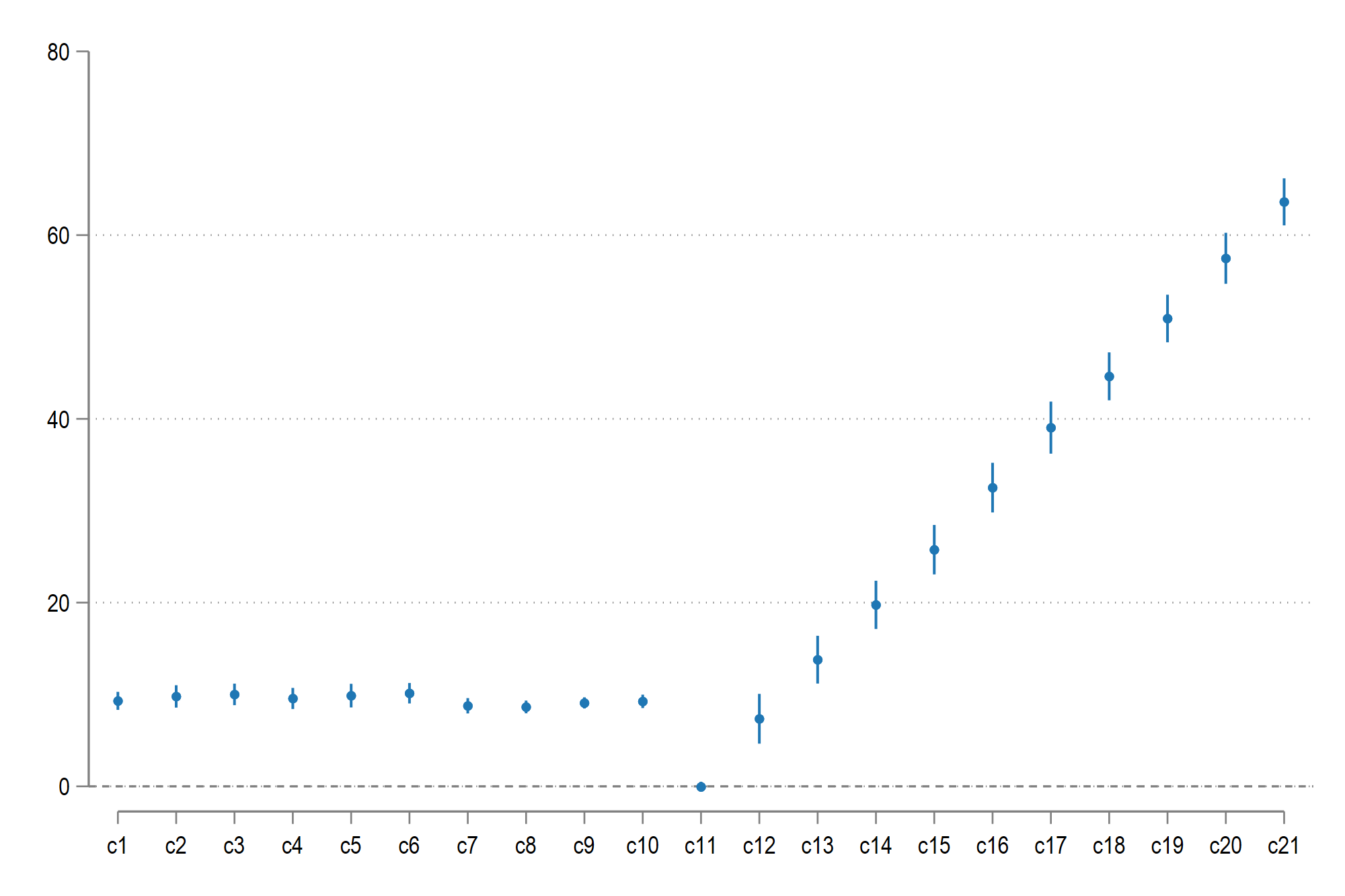
staggered Y, i(id) t(t) g(gvar) estimand(eventstudy) eventTime(-10/10)
and we get this output:
Some estimated variances < 0; setting to 0 as applicable.
(warning: e(V) is a diagonal matrix of SEs, not a full vcov matrix)

Staggered Treatment Effect Estimate                      Number of obs = 1,800

------------------------------------------------------------------------------
             |              Adjusted
             | Coefficient  std. err.      z    P>|z|     [95% conf. interval]
-------------+----------------------------------------------------------------
    gvar -10 |  -.1473483   .3229707    -0.46   0.648    -.7803593    .4856627
          -9 |  -.0430707    .299842    -0.14   0.886    -.6307503    .5446089
          -8 |   .0821222   .2862922     0.29   0.774    -.4790002    .6432445
          -7 |  -.2147896   .2869889    -0.75   0.454    -.7772775    .3476982
          -6 |  -.1826799   .2832417    -0.64   0.519    -.7378234    .3724636
          -5 |  -.2481264   .2436569    -1.02   0.309     -.725685    .2294323
          -4 |   -.003968   .2669453    -0.01   0.988    -.5271713    .5192352
          -3 |    -.20843   .2915786    -0.71   0.475    -.7799135    .3630536
          -2 |   .0561997   .4495108     0.13   0.901    -.8248253    .9372247
          -1 |   3.55e-15          .        .       .            .           .
           0 |  -.0439985   .2793774    -0.16   0.875    -.5915681    .5035711
           1 |   7.357605   1.382526     5.32   0.000     4.647904    10.06731
           2 |   13.78912   1.325263    10.40   0.000     11.19165    16.38658
           3 |   19.75595    1.33892    14.76   0.000     17.13171    22.38018
           4 |   25.76031   1.372833    18.76   0.000      23.0696    28.45101
           5 |   32.51529   1.378378    23.59   0.000     29.81371    35.21686
           6 |   39.04744   1.445284    27.02   0.000     36.21473    41.88014
           7 |   44.62738   1.330505    33.54   0.000     42.01964    47.23512
           8 |   50.92396   1.321695    38.53   0.000     48.33349    53.51444
           9 |   57.47601   1.415283    40.61   0.000     54.70211    60.24991
          10 |   63.62182   1.306207    48.71   0.000      61.0617    66.18193
------------------------------------------------------------------------------
Command results
Additional outputs show:
| Metric | Value |
|---|---|
| Sample size | 1,800 |
| Event time 0 | -0.0440 |
| Event time 1 | 7.3576 |
| Event time 5 | 32.5153 |
| Event time 10 | 63.6218 |
| Example lead at -2 | 0.0562 |
These additional diagnostics note that some estimated variances are set to zero and that e(V) is diagonal in this implementation.
Graph is generated following the process described here:
tempname CI b
mata st_matrix("`CI'", st_matrix("r(table)")[5::6, .])
mata st_matrix("`b'",  st_matrix("e(b)"))
coefplot matrix(`b'), ci(`CI') vertical yline(0)