hdidregress
Table of contents
Notes
hdidregressis a native Stata implementation of Callaway and Sant’Anna (2021).
Installation
Requires Stata 18 or higher. Take a look at the help file:
help hdidregress
Test the command
Please make sure that you generate the shared setup data using the setup block given here.
hdidregress aipw (Y) (D), group(id) time(t)
The paired dofile also demonstrates additional estimators and decomposition checks:
bacondecomp Y D
bacondecomp Y D, ddetail

hdidregress twfe (Y) (D), group(id) time(t)
hdidregress aipw (Y) (D), group(id) time(t)
hdidregress ipw (Y) (D), group(id) time(t)
hdidregress ra (Y) (D), group(id) time(t)
If you want to mirror the dofile workflow exactly, run the command block above before plotting so the comparison across estimators is reproducible from a single script.
Which gives us this output (truncated for visibility):
Computing decomposition across 5 timing groups
including a never-treated group
------------------------------------------------------------------------------
           Y | Coefficient  Std. err.      z    P>|z|     [95% conf. interval]
-------------+----------------------------------------------------------------
           D |   77.59101   3.731448    20.79   0.000     70.27751    84.90452
------------------------------------------------------------------------------

Bacon Decomposition

+---------------------------------------------------+
|                      |         Beta   TotalWeight |
|----------------------+----------------------------|
|        Timing_groups |  31.77318774   .4830876526 |
|       Never_v_timing |  120.4106995   .5169123474 |
+---------------------------------------------------+
Command results
Additional outputs show the same dataset and workflow:
| Metric | Value |
|---|---|
didregress ATET |
77.5910 |
| 95% CI | [54.8957, 100.2864] |
| Treated vs never component | 120.4107 (weight 0.5169) |
| Earlier vs later component | 88.1972 (weight 0.3332) |
| Later vs earlier component | -93.6920 (weight 0.1499) |
This decomposition context is useful when comparing TWFE-style averages to heterogeneity-robust estimators.
The command also has a built in graph option:
estat atetplot, sci
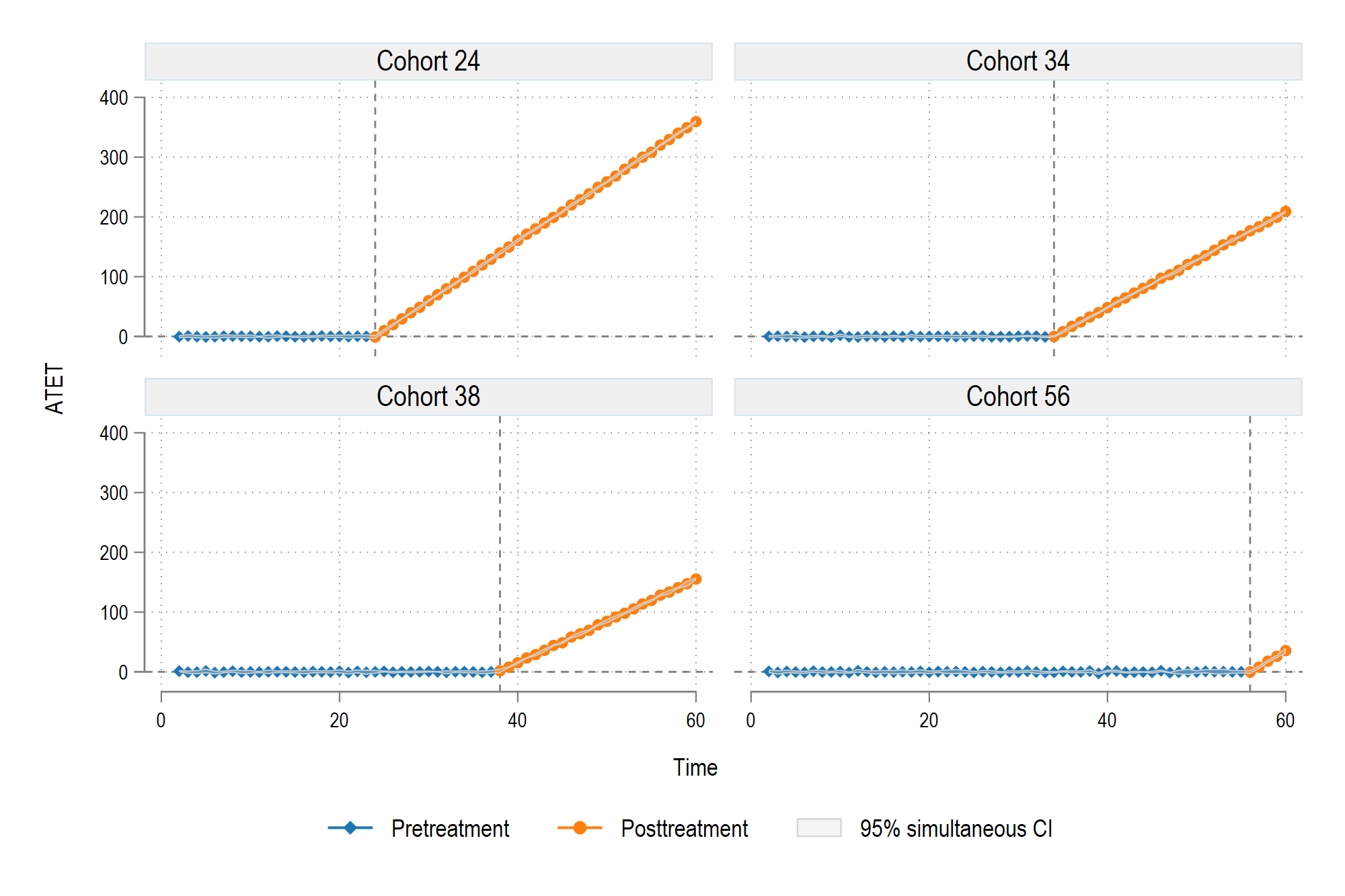
The command’s built-in graph option gives us:
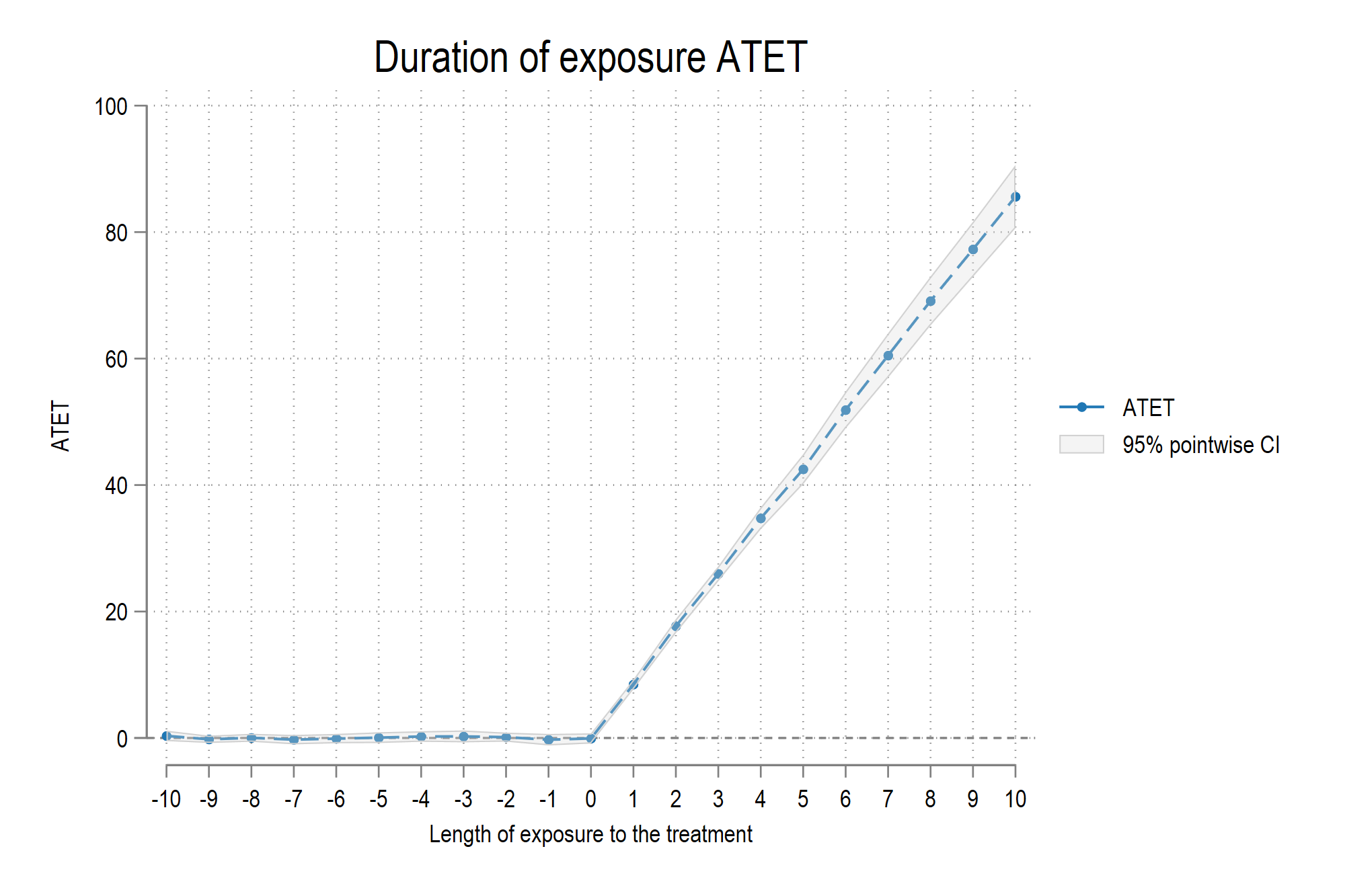
estat aggregation, dynamic(-10(1)10) graph