Stata code
This section is the Stata companion to the DiD methods covered on this site. Each page documents one estimator, including installation, a minimal test command, and an event-study style plot whenever supported.
How To Use This Section
- Start with the conceptual pages: TWFE and Bacon decomposition.
- Generate the common demo dataset once.
- Run the estimator pages one by one using the same data.
- Finish with the combined comparison page to visualize differences.
Shared Variable Notation
All Stata examples use the following symbols and naming convention:
| Symbol | Description |
|---|---|
| \(i\) | panel id variable |
| \(t\) | time variable |
| \(Y\) | outcome variable |
| \(D\) | treatment indicator (1 if treated, 0 otherwise) |
| \(gvar\) | first treatment cohort (0 for never treated when needed) |
| \(\epsilon_{it}\) | idiosyncratic error |
Common Workflow Assumptions
- Data are in panel format and typically set with
xtset id t. - Treatment can be staggered across cohorts.
- Several estimators require additional helper variables such as leads/lags,
first_treat,never_treat, andgvargenerated in the shared setup block below. - Commands from SSC evolve; examples reflect the last checked date on each estimator page.
Shared Data Setup
Use this one-time setup to generate the common sample dataset used in the Stata estimator pages.
clear

local units = 30
local start = 1
local end 	= 60

local time = `end' - `start' + 1
local obsv = `units' * `time'
set obs `obsv'

egen id	   = seq(), b(`time')
egen t 	   = seq(), f(`start') t(`end')

sort  id t
xtset id t


set seed 20211222

gen Y 	   		= 0		// outcome variable
gen D 	   		= 0		// intervention variable
gen cohort      = .  	// treatment cohort
gen effect      = .		// treatment effect size
gen first_treat = .		// when the treatment happens for each cohort
gen rel_time	= .     // time - first_treat

levelsof id, local(lvls)
foreach x of local lvls {
    local chrt = runiformint(0,5)
    replace cohort = `chrt' if id==`x'
}


levelsof cohort , local(lvls)
foreach x of local lvls {

    local eff = runiformint(2,10)
        replace effect = `eff' if cohort==`x'

    local timing = runiformint(`start',`end' + 20)	//
    replace first_treat = `timing' if cohort==`x'
    replace first_treat = . if first_treat > `end'
        replace D = 1 if cohort==`x' & t>= `timing'
}

replace rel_time = t - first_treat
replace Y = id + t + cond(D==1, effect * rel_time, 0) + rnormal()


// generate leads and lags (used in some commands)

summ rel_time
local relmin = abs(r(min))
local relmax = abs(r(max))

    // leads
    cap drop F_*
    forval x = 2/`relmin' {  // drop the first lead
        gen F_`x' = rel_time == -`x'
    }


    //lags
    cap drop L_*
    forval x = 0/`relmax' {
        gen L_`x' = rel_time ==  `x'
    }


// generate the control_cohort variables  (used in some commands)

gen never_treat = first_treat==.

sum first_treat
gen last_cohort = first_treat==r(max) // dummy for the latest- or never-treated cohort


// generate the gvar variables (used in some commands)
gen gvar = first_treat
recode gvar (. = 0)
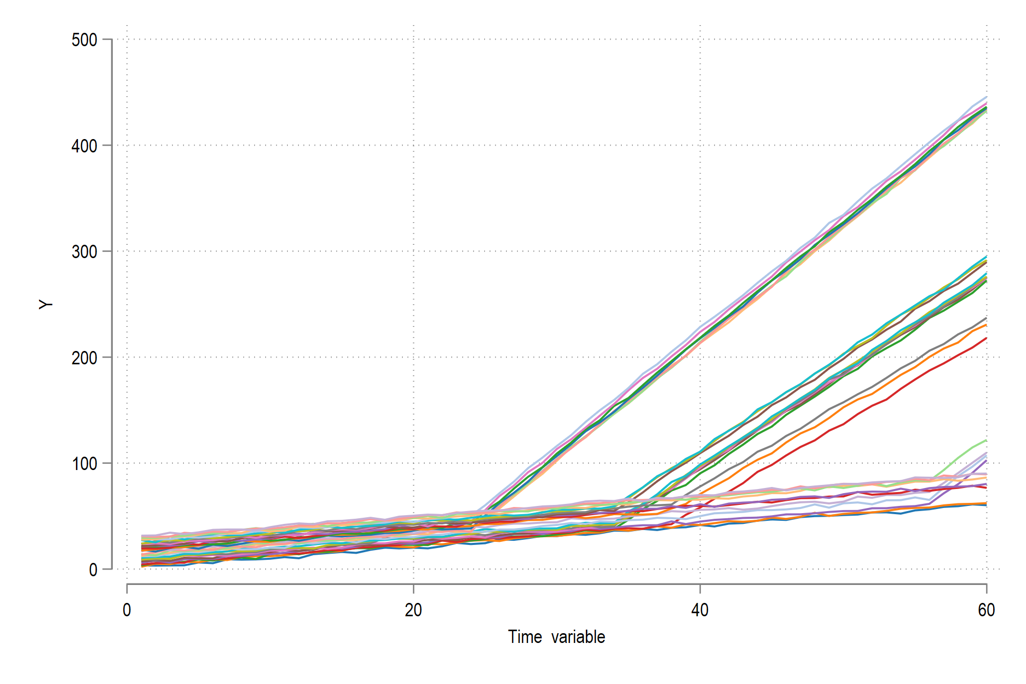
Generate the graph:
xtline Y, overlay legend(off)
Reproducibility Notes
- Keep your Stata version and package versions recorded when reproducing results.
- Use explicit random seeds when commands involve simulation or bootstrap steps.
- If two estimators disagree, first check assumptions and target estimands before comparing coefficients.
Related Section
R implementations are documented here: