The Twoway Fixed Effects (TWFE) model
Table of contents
- TOC
The classic 2x2 DiD or the Twoway Fixed Effects Model (TWFE)
We start with the classic Twoway Fixed Effects (TWFE) model:
\[y_{it} = \beta_0 + \beta_1 Treat_i + \beta_2 Post_t + \beta_3 Treat_i Post_t + \epsilon_{it}\]The 2x2 setup can be summarized with the following table:
| Treatment = 0 | Treatment = 1 | Difference | |
|---|---|---|---|
| Post = 0 | $\beta_0$ | $\beta_0 + \beta_1$ | $\beta_1$ |
| Post = 1 | $\beta_0 + \beta_2$ | $\beta_0 + \beta_1 + \beta_2 + \beta_3$ | $\beta_1 + \beta_3$ |
| Difference | $\beta_2$ | $\beta_2 + \beta_3$ | $\beta_3$ |
The triple difference estimator (DDD)
The triple-difference estimator (DDD) stacks one DD on top of another. You start with a treated and untreated group over time, and then compare that DD to a second, comparable group. In practice, this means there are two treatment dimensions: the main treatment and an additional comparison dimension that acts like a placebo contrast.
\[y_{it} = \beta_0 + \beta_1 P_{i} + \beta_2 C_{j} + \beta_3 T_t + \beta_4 (P_i T_t) + \beta_5 (C_j T_t) + \beta_6 (P_i C_j) + \beta_7 (P_i C_j T_t) + \epsilon_{it}\]Here we have 3x3 combinations: P = {0,1}, T = {0,1}, C = {0,1}. As in 2x2 DD, the key coefficient is $\beta_7$. Rather than writing one large table, it is easier to present results for $C = 0$ (main group) and $C = 1$ (comparison group). The difference between those two DDs is exactly $\beta_7$.
Main group ($C = 0$):
| T = 0 | T = 1 | Difference | |
|---|---|---|---|
| P = 0 | $\beta_0$ | $\beta_0 + \beta_3$ | $\beta_3$ |
| P = 1 | $\beta_0 + \beta_1$ | $\beta_0 + \beta_1 + \beta_3 + \beta_4$ | $\beta_3 + \beta_4$ |
| Difference | $\beta_1$ | $\beta_1 + \beta_4$ | $\beta_4$ |
Comparison group ($C = 1$):
| T = 0 | T = 1 | Difference | |
|---|---|---|---|
| P = 0 | $\beta_0 + \beta_2$ | $\beta_0 + \beta_2 + \beta_3 + \beta_5$ | $\beta_3 + \beta_5$ |
| P = 1 | $\beta_0 + \beta_1 + \beta_2 + \beta_6$ | $\beta_0 + \beta_1 + \beta_2 + \beta_3 + \beta_4 + \beta_5 + \beta_6 + \beta_7$ | $\beta_3 + \beta_4 + \beta_5 + \beta_7$ |
| Difference | $\beta_1 + \beta_6$ | $\beta_1 + \beta_4 + \beta_6 + \beta_7$ | $\beta_4 + \beta_7$ |
Let’s take the difference between the two matrices or (C = 1) - (C = 0):
| T = 0 | T = 1 | Difference | |
|---|---|---|---|
| P = 0 | $\beta_2$ | $\beta_2 + \beta_5$ | $\beta_5$ |
| P = 1 | $\beta_2 + \beta_6$ | $\beta_2 + \beta_5 + \beta_6 + \beta_7$ | $\beta_5 + \beta_7$ |
| Difference | $\beta_6$ | $\beta_6 + \beta_7$ | $\beta_7$ |
This final table makes it clear that the DDD estimand is $\beta_7$. In practice, this table-based view is much easier to read than listing expected values for all cells one by one.
The generic TWFE functional form
With multiple periods and many units, the 2x2 DD extends to:
\[y_{it} = \alpha_{i} + \alpha_t + \beta^{TWFE} D_{it} + \epsilon_{it}\]Stata Code
Let’s build a simple 2x2 example in Stata. First, define the panel structure. Since this is 2x2, we only need two units and two periods:
clear
local units = 2
local start = 1
local end   = 2

local time = `end' - `start' + 1
local obsv = `units' * `time'
set obs `obsv'

egen id	   = seq(), b(`time')
egen t 	   = seq(), f(`start') t(`end')

sort id t
xtset id t

lab var id "Panel variable"
lab var t  "Time  variable"
Next, define treatment and a clean outcome equation without random noise:
gen D = id==2 & t==2

gen btrue = cond(D==1, 2, 0)
	gen Y = id + 3*t + btrue*D
From the last line, treatment should raise Y by 2 units for the treated unit in the post period. We can verify that in a plot:
lab de prepost 1 "Pre" 2 "Post"
lab val t prepost

twoway ///
	(connected Y t if id==1) ///
	(connected Y t if id==2) ///
		,	///
		legend(order(1 "id=1" 2 "id=2")) ///
		xlabel(1 2, valuelabel) ylabel(4(1)10)
This produces:
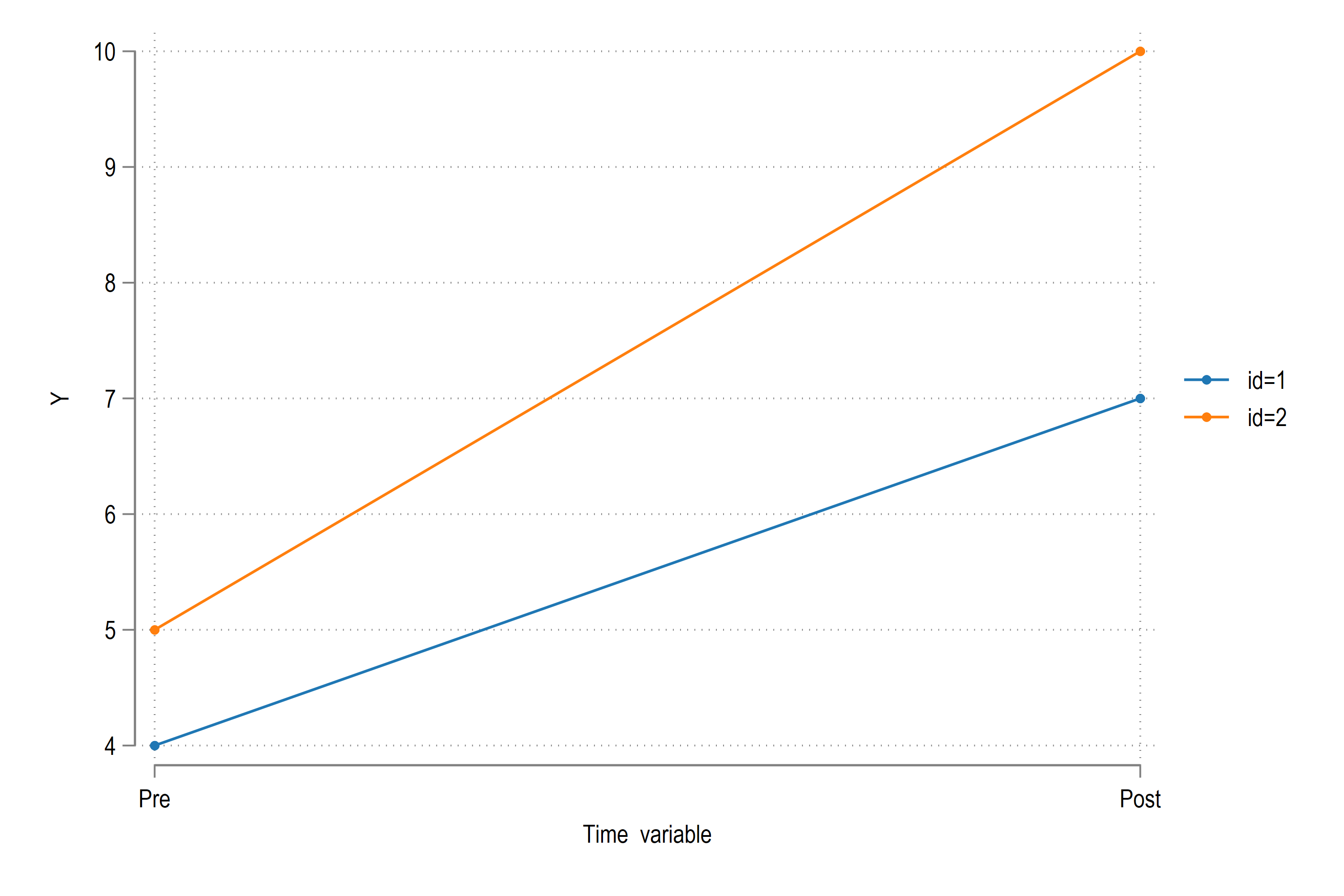
The gap between the two lines is 1 in the pre period and 3 in the post period, so the DD is 2, exactly as coded.
We can recover the same result from a panel regression:
xtset id t
xtreg Y D t, fe
In the regression output, the coefficient on D is
\[\beta^{TWFE} = 2\]. You can get the same result with reghdfe, which we use again below:
reghdfe Y D, absorb(id t)
which again gives us the same result for the D coefficient. You can also estimate the same design as OLS with explicit fixed effects:
reg Y i.id i.t D
The output again recovers $\hat\beta_D = 2$ and a post-period time effect of 3, matching the data-generating process.
Adding more time periods
Now extend the same setup to 10 periods per unit:
clear
local units = 2
local start = 1
local end 	= 10

local time = `end' - `start' + 1
local obsv = `units' * `time'
set obs `obsv'

egen id	   = seq(), b(`time')
egen t 	   = seq(), f(`start') t(`end')

sort  id t
xtset id t

lab var id "Panel variable"
lab var t  "Time  variable"
Use a simple treatment path: unit 2 is treated from period 5 onward with an effect of 3:
gen D = id==2 & t>=5
lab var D "Treated"

gen btrue = cond(D==1, 3, 0)

gen Y = id + t +  btrue*D
lab var Y "Outcome variable"
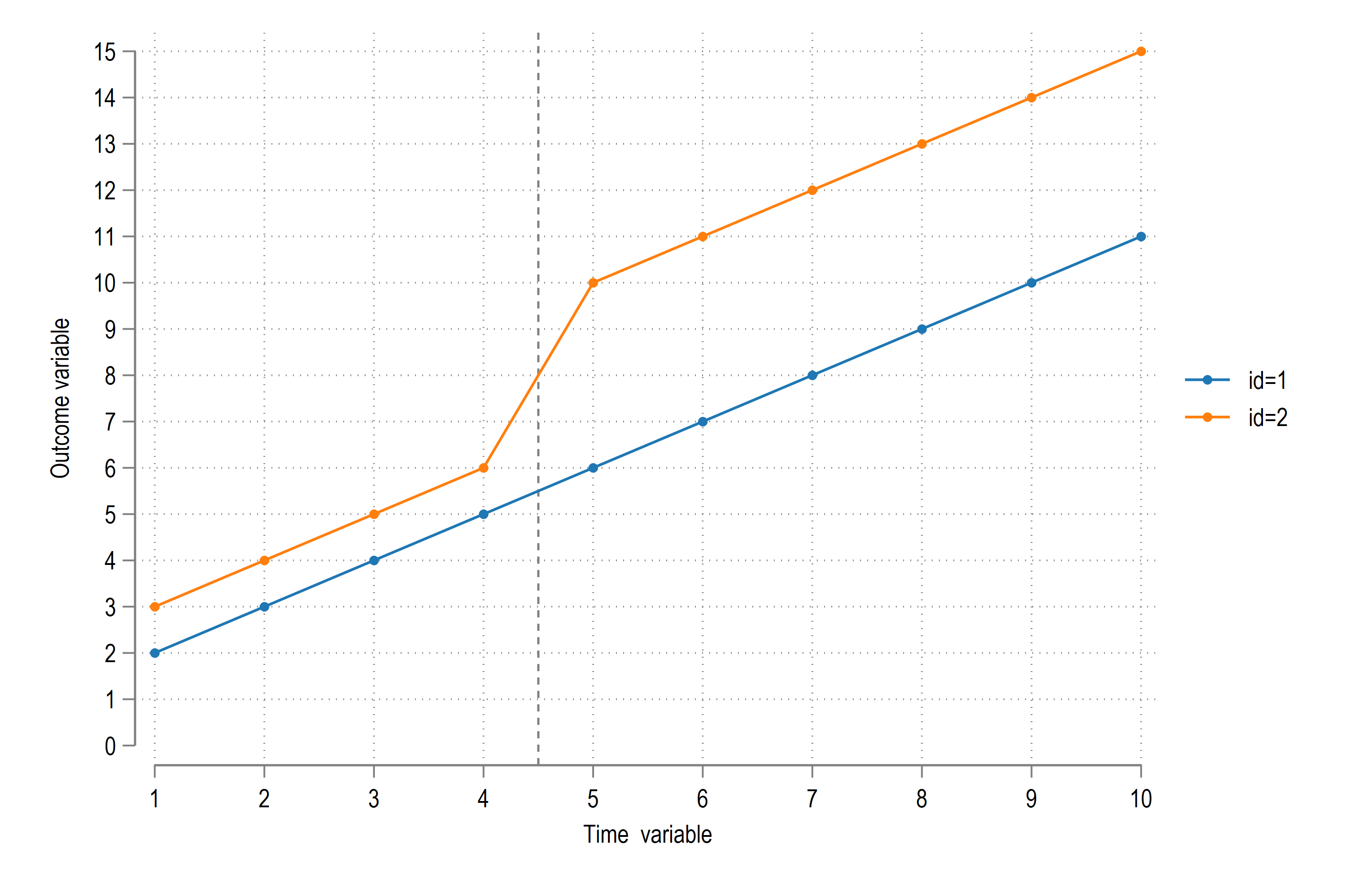
The pattern is easy to see in the following plot:
Run:
xtreg Y D t, fe
reghdfe Y D, absorb(id t)
xtreg shows that $t$ increases Y by about 1 unit per period, as expected. The intercept is 1.5 (the average implied baseline at
$t=0$ across both units), and $\beta^{TWFE} = 3$, the true treatment effect.
Using the table output (table P id, stat(mean Y)), the manual DD in this setup is:
which is identical to the regression coefficient.
More units, same treatment time, different treatment effects
Now consider one control group and two treated groups. Both treated groups start at the same time, but with different treatment intensities:
clear
local units = 3
local start = 1
local end 	= 10

local time = `end' - `start' + 1
local obsv = `units' * `time'
set obs `obsv'

egen id	   = seq(), b(`time')
egen t 	   = seq(), f(`start') t(`end')

lab var id "Panel variable"
lab var t  "Time  variable"

sort  id t
xtset id t


gen D = 0
replace D = 1 if id>=2 & t>=5
lab var D "Treated"

cap drop Y
gen Y = 0
replace Y = cond(D==1, 2, 0) if id==2
replace Y = cond(D==1, 4, 0) if id==3

lab var Y "Outcome variable"
and plot it:
twoway ///
	(connected Y t if id==1) ///
	(connected Y t if id==2) ///
	(connected Y t if id==3) ///
		,	///
		xline(4.5) ///
		xlabel(1(1)10) ///
		legend(order(1 "id=1" 2 "id=2" 3 "id=3"))
from which we get:
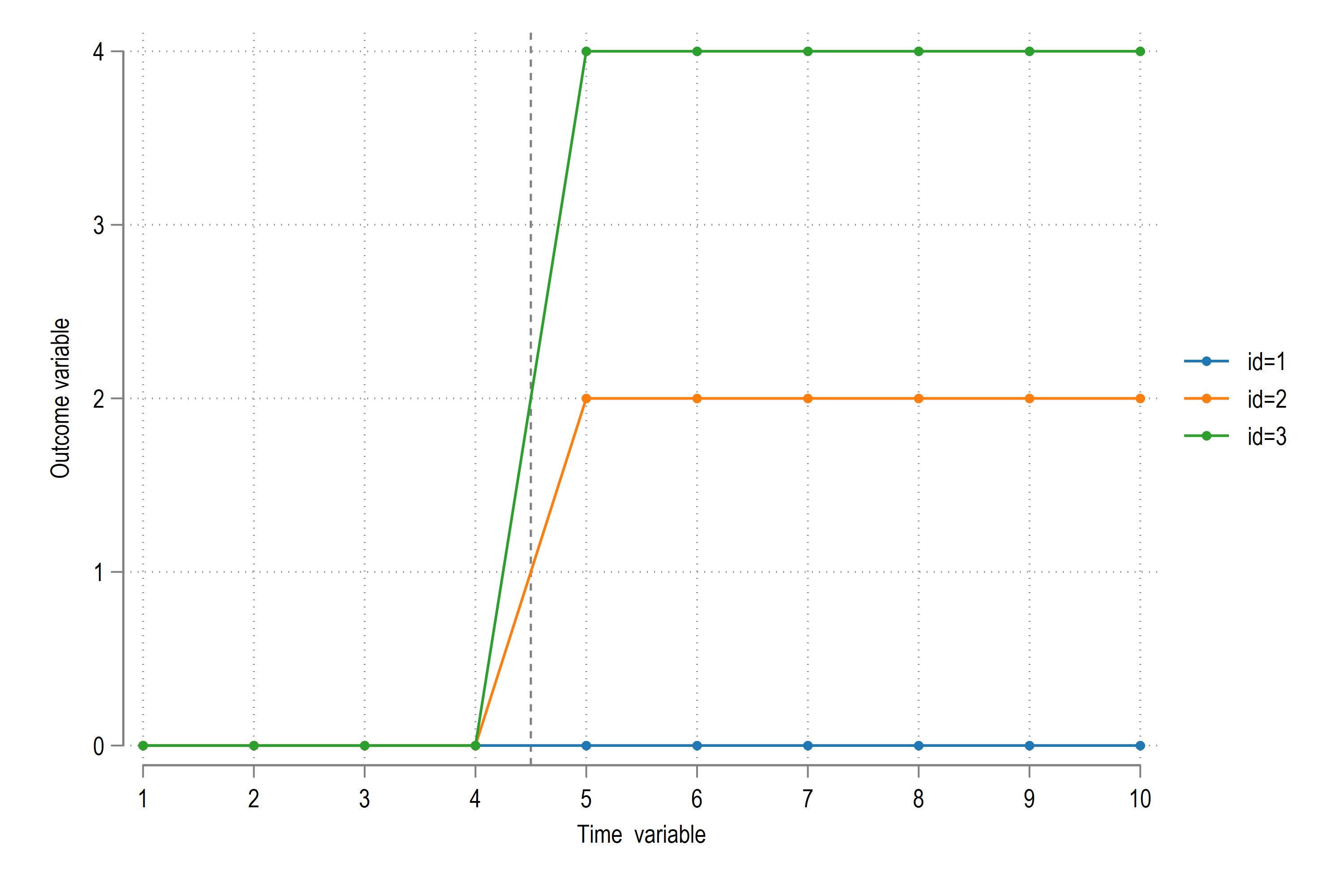
The post-treatment effect is 2 for id=2 and 4 for id=3, so the average effect is 3. We can verify this directly in regression:
xtreg Y D t, fe
In this stripped-down version, the average effect is easy to see from the graph. Once we add unit and time components, visual inspection is less informative. Here is the full code:
clear
local units = 3
local start = 1
local end 	= 10

local time = `end' - `start' + 1
local obsv = `units' * `time'
set obs `obsv'

egen id	   = seq(), b(`time')
egen t 	   = seq(), f(`start') t(`end')

sort  id t
xtset id t

lab var id "Panel variable"
lab var t  "Time  variable"

gen D = 0
replace D = 1 if id>=2 & t>=5
lab var D "Treated"

cap drop Y
gen Y = 0
replace Y = id + t + cond(D==1, 0, 0) if id==1
replace Y = id + t + cond(D==1, 2, 0) if id==2
replace Y = id + t + cond(D==1, 4, 0) if id==3

lab var Y "Outcome variable"

twoway ///
	(connected Y t if id==1) ///
	(connected Y t if id==2) ///
	(connected Y t if id==3) ///
		,	///
		xline(4.5) ///
		xlabel(1(1)10) ///
		legend(order(1 "id=1" 2 "id=2" 3 "id=3"))
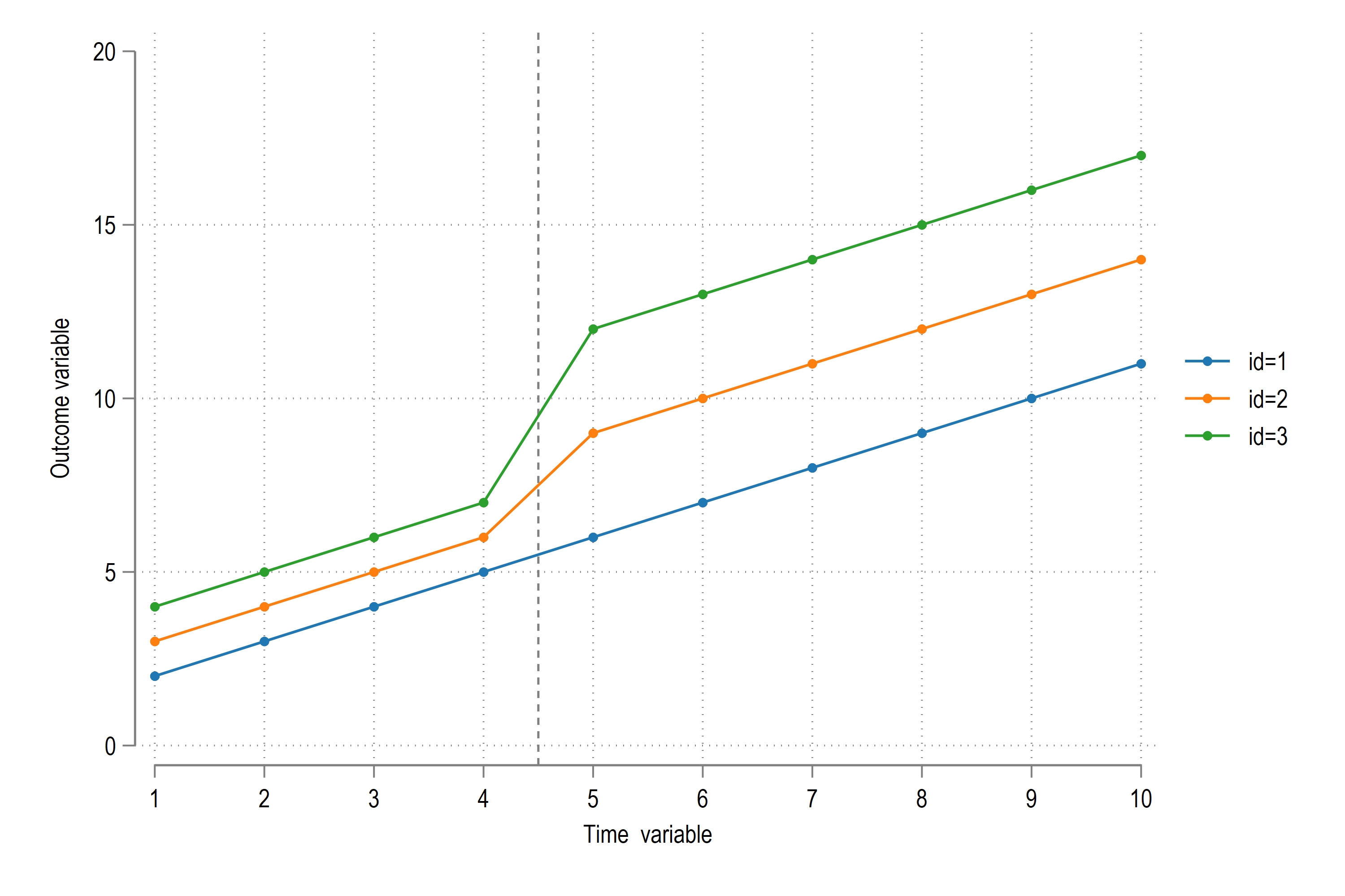
As before, the ATT is $\beta^{TWFE}=3$, but it is no longer obvious from the raw plot because unit and time patterns are mixed in. Rather than partialling out by hand, we estimate:
xtreg Y D t, fe
which returns ATT = 3, the average of the two treatment effects.
The key point is that accounting for unit and time effects is essential for a valid DD comparison. If these are omitted, the treatment coefficient can be far off. Compare:
reg Y D           // not controlling for any effects
reg Y D i.t       // only time fixed effects
reg Y D i.id      // only panel fixed effects
reg Y D i.t i.id  // panel and time fixed effects (correct!)
Additional outputs show these values:
reg Y D: $\hat\beta_D = 7.17$reg Y D i.t: $\hat\beta_D = 4.5$reg Y D i.id: $\hat\beta_D = 8.0$reg Y D i.t i.id: $\hat\beta_D = 3.0$
| Specification | Time FE | Unit FE | Estimate on D |
|---|---|---|---|
reg Y D |
No | No | 7.1667 |
reg Y D i.t |
Yes | No | 4.5000 |
reg Y D i.id |
No | Yes | 8.0000 |
reg Y D i.t i.id |
Yes | Yes | 3.0000 |
This is a good reminder that leaving out one or both fixed effects can seriously distort the treatment estimate.
More units, differential treatment time, different treatment effects
Now we move to staggered adoption where groups are treated at different times. We again use a generated dataset and then recover $\beta^{TWFE}$ through regression with fixed effects:
clear
local units = 3
local start = 1
local end 	= 10

local time = `end' - `start' + 1
local obsv = `units' * `time'
set obs `obsv'

egen id	   = seq(), b(`time')
egen t 	   = seq(), f(`start') t(`end')

sort  id t
xtset id t

lab var id "Panel variable"
lab var t  "Time  variable"

gen D = 0
replace D = 1 if id==2 & t>=5
replace D = 1 if id==3 & t>=8
lab var D "Treated"

gen Y = 0
replace Y = D * 2 if id==2 & t>=5
replace Y = D * 4 if id==3 & t>=8

lab var Y "Outcome variable"


twoway ///
	(connected Y t if id==1) ///
	(connected Y t if id==2) ///
	(connected Y t if id==3) ///
		,	///
		xline(4.5 7.5) ///
		xlabel(1(1)10) ///
		legend(order(1 "id=1" 2 "id=2" 3 "id=3"))
This produces the following figure:
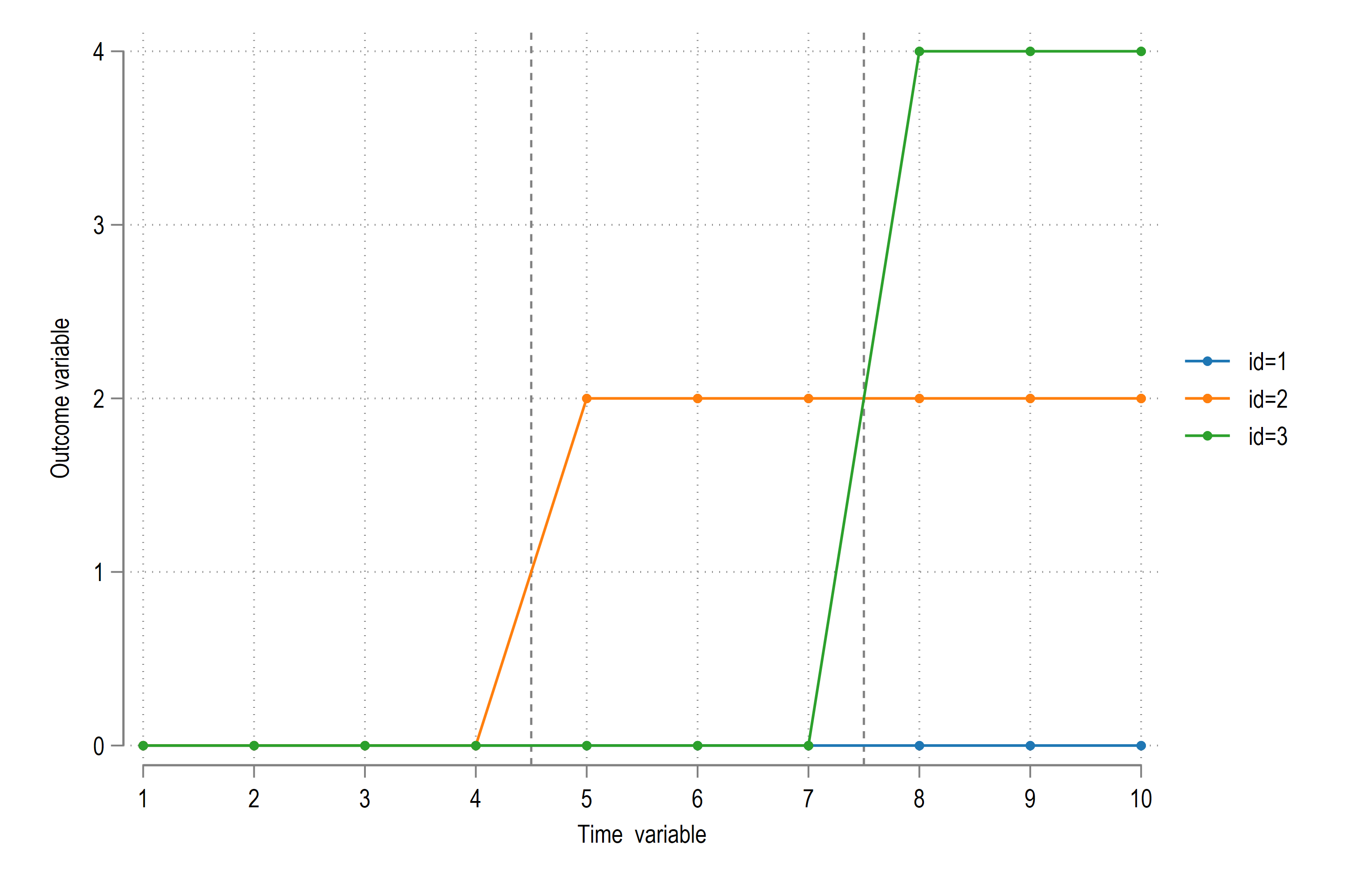
In this figure, id=2 is treated from $t=5$ onward, while id=3 is treated from $t=8$ onward. So what is ATT in this case?
Unlike the earlier examples, you cannot read ATT cleanly from the graph. With staggered timing, treatment comparisons vary across cohorts and periods. To recover ATT, we need to net out both unit and time effects.
We can do these regressions to see the outcomes:
reg Y D            // not controlling for any effects
reg Y D i.t        // only time fixed effects
reg Y D i.id       // only panel fixed effects
reg Y D i.t i.id   // panel and time fixed effects (correct!)
The estimates in the log are:
reg Y D, robust: $\hat\beta_D = 2.6667$reg Y D i.t, robust: $\hat\beta_D = 2.5$reg Y D i.id, robust: $\hat\beta_D = 2.9333$reg Y D i.t i.id, robust: $\hat\beta_D = 2.9091$
| Specification | Time FE | Unit FE | Robust? | Estimate on D |
|---|---|---|---|---|
reg Y D |
No | No | Yes | 2.6667 |
reg Y D i.t |
Yes | No | Yes | 2.5000 |
reg Y D i.id |
No | Yes | Yes | 2.9333 |
reg Y D i.t i.id |
Yes | Yes | Yes | 2.9091 |
The last specification gives the TWFE estimate, $\beta^{TWFE} \approx 2.91$. This is an FE-weighted average after removing unit and time effects.
You can recover the same estimate using:
xtreg Y D i.t, fe
reghdfe Y D, absorb(id t)
Both commands return the same estimate, $\beta^{TWFE} = 2.91$.
Important: with staggered treatment, we need to use full time fixed effects (i.t), not a single linear trend (t):
xtreg Y D i.t, fe robust
Why is this happening? Because with staggered timing and heterogeneous effects, “pre/post” and “treated/untreated” are not single comparisons anymore. In $5 \leq t < 8$, only id=2 contributes new treatment variation. For $t \geq 8$, id=3 begins treatment while id=2 is already treated.
That is why the simple average among treated observations, $\frac{2 \times 6 + 4 \times 3}{9} = 2.6667$, does not equal the TWFE estimate of 2.9091.
Bacon decomposition
To see exactly where the TWFE estimate is coming from, we can break it into its 2x2 DD components using Bacon decomposition:
bacondecomp Y D, ddetail
gives these 2x2 components:
- Early vs Late: estimate = 2.0000, weight = 0.1818
- Late vs Early: estimate = 4.0000, weight = 0.1364
- Never vs Timing: estimate = 2.9333, weight = 0.6818
| Component | 2x2 Estimate | Weight |
|---|---|---|
| Early vs Late | 2.0000 | 0.1818 |
| Late vs Early | 4.0000 | 0.1364 |
| Never vs Timing | 2.9333 | 0.6818 |
The TWFE coefficient is the weighted average of these components:
\[2.9091 \approx 0.1818\times2.0000 + 0.1364\times4.0000 + 0.6818\times2.9333.\]In this example, most identifying weight comes from treated-vs-never comparisons.
We discuss this in detail in Bacon decomposition.