stackedev
Table of contents
Notes
- Based on: Cengiz, Dube, Lindner, Zipperer 2019. The effect of minimum wages on low-wage jobs
- Program version (if available): -
- Last checked: 7 Jul 2026
The dofile defines untreated units with no_treat, so the estimation call below uses never_treat(no_treat).
Installation and options
Install the command from SSC:
ssc install stackedev, replace
Take a look at the help file:
help stackedev
Test the command
Define the reference year:
ren F_1 ref //base year
Let’s run the basic stackedev command:
stackedev Y F_* L_* ref, cohort(first_treat) time(t) never_treat(no_treat) unit_fe(id) clust_unit(id)
which will show this output:
**** Building Stack 24 ****
**** Building Stack 34 ****
**** Building Stack 38 ****
**** Building Stack 56 ****
**** Appending Stacks ****
**** Estimating Model with reghdfe ****
(MWFE estimator converged in 2 iterations)
note: ref omitted because of collinearity
warning: missing F statistic; dropped variables due to collinearity or too few clusters

HDFE Linear regression                            Number of obs   =      3,060
Absorbing 2 HDFE groups                           F(  91,     49) =          .
Statistics robust to heteroskedasticity           Prob > F        =          .
                                                  R-squared       =     0.9974
                                                  Adj R-squared   =     0.9970
                                                  Within R-sq.    =     0.9896
Number of clusters (unit_stack) =         50      Root MSE        =     4.1325

                            (Std. err. adjusted for 50 clusters in unit_stack)
------------------------------------------------------------------------------
             |               Robust
           Y | Coefficient  std. err.      t    P>|t|     [95% conf. interval]
-------------+----------------------------------------------------------------
         F_2 |   .2173356    .429718     0.51   0.615    -.6462151    1.080886
         F_3 |   .1386198   .4137917     0.33   0.739    -.6929257    .9701654
         F_4 |  -.0771335   .4251788    -0.18   0.857    -.9315624    .7772953
         F_5 |  -.3127445   .3628929    -0.86   0.393    -1.042005    .4165161
         F_6 |  -.4361147   .4095256    -1.06   0.292    -1.259087    .3868578
         F_7 |  -.3144571    .526613    -0.60   0.553    -1.372726    .7438113
         F_8 |  -.1044745   .4800377    -0.22   0.829    -1.069146    .8601974
         F_9 |  -.1156501   .4238786    -0.27   0.786    -.9674661    .7361659
        F_10 |   .1485313   .4001261     0.37   0.712    -.6555522    .9526148
        F_11 |  -.2473913     .47278    -0.52   0.603    -1.197478    .7026957
        F_12 |  -.1452927   .4785819    -0.30   0.763    -1.107039    .8164536
        F_13 |   .1286208   .4821393     0.27   0.791    -.8402744    1.097516
        F_14 |   .1440072   .3947098     0.36   0.717    -.6491919    .9372063
        F_15 |   .3114543    .476962     0.65   0.517    -.6470368    1.269945
        F_16 |   .1721978   .5333658     0.32   0.748    -.8996409    1.244037
        F_17 |  -.7585561   .3663682    -2.07   0.044    -1.494801   -.0223118
        F_18 |   .0699152   .5175897     0.14   0.893    -.9702202    1.110051
        F_19 |  -.3875619   .2815699    -1.38   0.175    -.9533978     .178274
        F_20 |   .0638705   .4198326     0.15   0.880    -.7798146    .9075557
        F_21 |    .035372   .4097576     0.09   0.932    -.7880668    .8588108
        F_22 |  -.5763502   .4471311    -1.29   0.203    -1.474894    .3221933
        F_23 |   .1005642   .3572709     0.28   0.780    -.6173985     .818527
        F_24 |   4.715301   .9921569     4.75   0.000     2.721487    6.709115
        F_25 |   3.848972   .9570067     4.02   0.000     1.925795    5.772149
        F_26 |   3.885843   .9759061     3.98   0.000     1.924686    5.846999
        F_27 |   3.665572   .9574264     3.83   0.000     1.741551    5.589592
        F_28 |   3.629329   .9877625     3.67   0.001     1.644346    5.614312
        F_29 |   4.376366   .9749251     4.49   0.000      2.41718    6.335551
        F_30 |    4.38623   .9937478     4.41   0.000     2.389219    6.383241
        F_31 |    3.95357   .9964798     3.97   0.000     1.951069    5.956071
        F_32 |   4.131159   .9566808     4.32   0.000     2.208637    6.053681
        F_33 |   4.421442   .9615812     4.60   0.000     2.489073    6.353812
        F_34 |   3.870751   1.112861     3.48   0.001     1.634373     6.10713
        F_35 |   3.975567   1.073438     3.70   0.001     1.818414    6.132721
        F_36 |   3.999014   1.177784     3.40   0.001     1.632169     6.36586
        F_37 |   3.909786   .9581247     4.08   0.000     1.984363     5.83521
        F_38 |   .9388715   .8728544     1.08   0.287    -.8151952    2.692938
        F_39 |   1.211486   .7498948     1.62   0.113    -.2954839    2.718456
        F_40 |   1.025343   .8874642     1.16   0.254    -.7580827     2.80877
        F_41 |   1.526626    .606473     2.52   0.015     .3078726    2.745379
        F_42 |   1.434986   .8133947     1.76   0.084     -.199592    3.069564
        F_43 |   2.300906   .5985228     3.84   0.000      1.09813    3.503683
        F_44 |   2.221324   .7714936     2.88   0.006     .6709491    3.771698
        F_45 |   .4473907   .6918146     0.65   0.521    -.9428628    1.837644
        F_46 |   1.606906   .5320911     3.02   0.004      .537629    2.676183
        F_47 |   1.220467     .99843     1.22   0.227    -.7859536    3.226887
        F_48 |    1.43739   .6826501     2.11   0.040     .0655537    2.809227
        F_49 |   1.691145   .6603621     2.56   0.014     .3640975    3.018192
        F_50 |   .5937526   .5885007     1.01   0.318    -.5888838    1.776389
        F_51 |   1.543893   .5838527     2.64   0.011      .370597    2.717189
        F_52 |   1.815931   .5872599     3.09   0.003      .635788    2.996074
        F_53 |   1.176133    .679497     1.73   0.090    -.1893669    2.541634
        F_54 |   2.117263   .9070423     2.33   0.024     .2944931    3.940032
        F_55 |   1.314801   .5422668     2.42   0.019     .2250752    2.404527
         L_0 |   .0100481    .498877     0.02   0.984    -.9924828    1.012579
         L_1 |   8.452976   .4244544    19.91   0.000     7.600003    9.305949
         L_2 |   17.61775   .4799071    36.71   0.000     16.65334    18.58216
         L_3 |   25.91892   .5228491    49.57   0.000     24.86822    26.96962
         L_4 |   34.59866   .8042661    43.02   0.000     32.98243    36.21489
         L_5 |   41.79543   1.039745    40.20   0.000     39.70599    43.88488
         L_6 |   51.13859   1.248299    40.97   0.000     48.63004    53.64715
         L_7 |   59.47399   1.577942    37.69   0.000     56.30299    62.64498
         L_8 |   68.24786   1.654616    41.25   0.000     64.92278    71.57293
         L_9 |   76.25018   1.923937    39.63   0.000     72.38389    80.11648
        L_10 |   84.44234   2.230286    37.86   0.000     79.96041    88.92427
        L_11 |   92.93716   2.283911    40.69   0.000     88.34747    97.52685
        L_12 |   102.2659   2.653712    38.54   0.000      96.9331    107.5988
        L_13 |    109.776   2.872513    38.22   0.000     104.0034    115.5485
        L_14 |   118.1795   3.204707    36.88   0.000     111.7394    124.6196
        L_15 |   127.3586   3.358882    37.92   0.000     120.6086    134.1085
        L_16 |   136.1793   3.598478    37.84   0.000     128.9479    143.4107
        L_17 |   144.5375    4.00305    36.11   0.000     136.4931     152.582
        L_18 |   153.3496   3.928038    39.04   0.000     145.4559    161.2433
        L_19 |    161.894   4.237581    38.20   0.000     153.3783    170.4098
        L_20 |   170.1305   4.407902    38.60   0.000     161.2725    178.9885
        L_21 |    177.795   4.631182    38.39   0.000     168.4883    187.1017
        L_22 |   187.4496   4.907435    38.20   0.000     177.5878    197.3115
        L_23 |   202.3896   4.333513    46.70   0.000     193.6811    211.0981
        L_24 |    211.301   4.491664    47.04   0.000     202.2746    220.3273
        L_25 |   220.5574   4.807412    45.88   0.000     210.8965    230.2182
        L_26 |   230.0163   4.752343    48.40   0.000     220.4661    239.5665
        L_27 |   258.8725   1.506249   171.87   0.000     255.8456    261.8994
        L_28 |   270.2441   1.502177   179.90   0.000     267.2253    273.2628
        L_29 |   280.5032   1.489283   188.35   0.000     277.5104     283.496
        L_30 |   290.4652   1.590089   182.67   0.000     287.2698    293.6606
        L_31 |   298.6743   1.470175   203.16   0.000     295.7199    301.6288
        L_32 |   310.7671    1.43449   216.64   0.000     307.8844    313.6498
        L_33 |   319.9876   1.486439   215.27   0.000     317.0004    322.9747
        L_34 |    330.728   1.523338   217.11   0.000     327.6668    333.7893
        L_35 |   339.7674   1.475247   230.31   0.000     336.8028     342.732
        L_36 |   349.8512    1.53732   227.57   0.000     346.7618    352.9405
         ref |          0  (omitted)
       _cons |   47.28654   .5001833    94.54   0.000     46.28138    48.29169
------------------------------------------------------------------------------

Absorbed degrees of freedom:
-----------------------------------------------------+
 Absorbed FE | Categories  - Redundant  = Num. Coefs |
-------------+---------------------------------------|
    id#stack |        51          51           0    *|
     t#stack |       240           1         239     |
-----------------------------------------------------+
* = FE nested within cluster; treated as redundant for DoF computation
Command results
Additional diagnostics show key values:
| Metric | Value |
|---|---|
| Estimation sample | 3,060 |
On-impact effect (L_0) |
0.0100 |
First post period (L_1) |
8.4530 |
Tenth post period (L_10) |
84.4423 |
Example lead (F_17) |
-0.7586 |
This run also reports a collinearity note for ref, which is expected because that period is the omitted baseline.
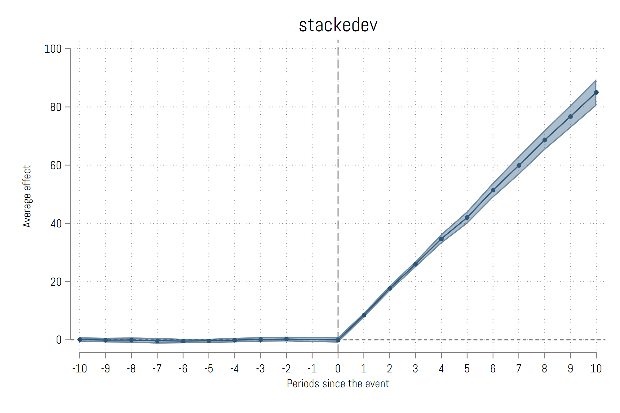
In order to plot the estimates we can use the event_plot (ssc install event_plot, replace) command where we restrict the figure to 10 leads and lags:
	event_plot, default_look graph_opt(xtitle("Periods since the event") ytitle("Average effect") xlabel(-10(1)10) ///
		title("stackedev")) stub_lag(L_#) stub_lead(F_#) trimlag(10) trimlead(10) together
And we get: