jwdid
Table of contents
Notes
- Based on: Wooldridge (2021). ETWFE-style DiD with staggered timing.
-
Program version (if available): v2.00 Paper Out
- Last checked: 7 Jul 2026
Installation and options
ssc install jwdid, replace
ssc install hdfe, replace // dependency
Take a look at the help file:
help jwdid
Test the command
Please make sure that you generate the shared setup data using the setup block given here
Let’s try the basic jwdid command:
jwdid Y, ivar(id) time(t) gvar(gvar) never
which should show this output:
WARNING: Singleton observations not dropped; statistical significance is biased (link)
(MWFE estimator converged in 2 iterations)
warning: missing F statistic; dropped variables due to collinearity or too few clusters

HDFE Linear regression                            Number of obs   =      1,800
Absorbing 2 HDFE groups                           F( 236,     29) =          .
Statistics robust to heteroskedasticity           Prob > F        =          .
                                                  R-squared       =     0.9999
                                                  Adj R-squared   =     0.9999
                                                  Within R-sq.    =     0.9996
Number of clusters (id)      =         30         Root MSE        =     1.0111

                                       (Std. err. adjusted for 30 clusters in id)
---------------------------------------------------------------------------------
                |               Robust
              Y | Coefficient  std. err.      t    P>|t|     [95% conf. interval]
----------------+----------------------------------------------------------------
gvar#t#c.__tr__ |
         24  1  |  -.3046101   .6300019    -0.48   0.632    -1.593109    .9838884
         24 24  |  -.9183905   .9302745    -0.99   0.332    -2.821015    .9842344
         24 25  |   9.725702   .8483403    11.46   0.000     7.990651    11.46075
         24 30  |    59.8352    .656269    91.17   0.000     58.49298    61.17742
         34 35  |    7.92487   .8199465     9.67   0.000     6.247891    9.601849
         38 39  |   7.982207   .4647076    17.18   0.000     7.031773    8.932641
         56 57  |   7.908278   .8946205     8.84   0.000     6.078574    9.737983

... output truncated ...
Command results
Additional diagnostics show key values:
| Metric | Value |
|---|---|
| Estimation sample | 1,800 |
Clusters (id) |
30 |
Example pre period (24 1) |
-0.3046 |
First strong post period (24 25) |
9.7257 |
Later post period (24 30) |
59.8352 |
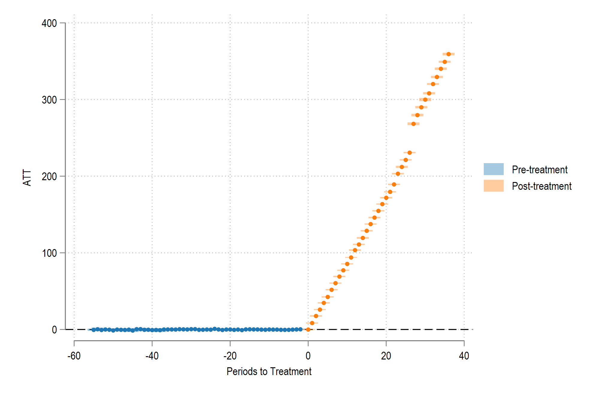
The dynamic path for treated cohorts is consistent with the increasing treatment effect in the data-generating process.
The command’s built-in graph option gives us:
estat event,  estore(jw)

jwdid_plot