fixest::sunab (Sun and Abraham 2020)
Table of contents
Introduction
Among (many) other things,
Laurent Bergé’s
fixest package supports the estimation
procedure described by the Sun and Abraham 2020 paper Estimating Dynamic
Treatment Effects in Event Studies with Heterogeneous Treatment
Effects
(hereafter SA20). The key function is
sunab(),
which provides equivalent
functionality to the eventstudyinteract Stata command. However, it requires
less manual tuning (e.g., leads and lags are detected automatically) and it
integrates natively with fixest’s other facilities (e.g. graphing and
tabling). As one would expect of fixest, estimation is also very fast—you
will likely find it to be the fastest option among all of the specialist DiD
libraries that we cover here. These features combine to make it an attractive
and natural option for staggered DiD settings.
Installation and options
The package can be installed from CRAN.
install.packages("fixest") # Install (only need to run once or when updating)
library("fixest")          # Load the package into memory (required each new session)
The key function for implementing the SA20 aggregation procedure is sunab().
This serves as an internal argument for the fixest::feols() function that
many users will be familiar with for estimating (high-dimensional fixed-effect)
regressions. The most basic form is thus:
feols(y ~ sunab(cohort, period) | id + period, data, ...)
where
| Variable | Description |
|---|---|
| y | outcome variable |
| cohort | variable describing a common treatment period (e.g., year_treated) |
| period | time variable |
| id | panel id |
| … | Additional arguments |
All of the regular feols() functionality and post-estimation options can be
layered on top of the basic case above. For example, users can add covariates,
change the default cohort reference (here: the never-treated), etc. It’s even
possible to integrate sunab() into fixest’s nonlinear model estimators
like feglm() and fepois(), although I don’t believe these have good
theoretical support. See the helpfile
(?sunab)
for more detailed information, as well as the
introductory vignette.
Dataset
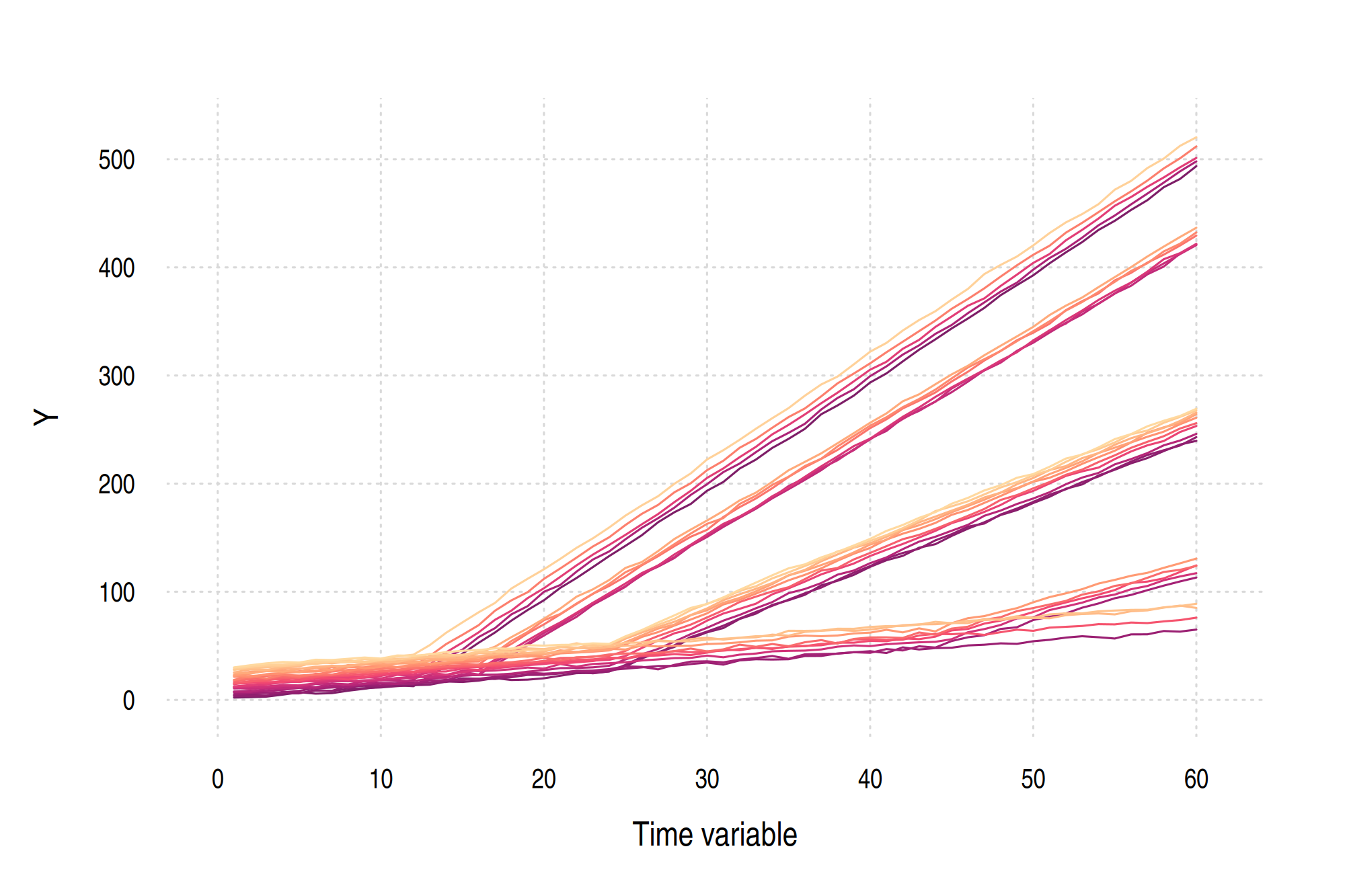
To demonstrate the package in action, we’ll use the fake dataset generated in the shared setup block here. Here’s a reminder of what the data look like.
head(dat)
#>   time id        y rel_time treat first_treat
#> 1    1  1 2.158289      -11 FALSE          12
#> 2    2  1 2.498052      -10 FALSE          12
#> 3    3  1 3.034077       -9 FALSE          12
#> 4    4  1 4.886266       -8 FALSE          12
#> 5    5  1 7.085950       -7 FALSE          12
#> 6    6  1 5.788352       -6 FALSE          12
Or, in graph form.
Test the package
Remember to load the package (if you haven’t already).
library(fixest)
Let’s try the basic sunab() function (as integrated inside feols()). Note
that we don’t have any covariates, although these would be trivial to add to the
model formula. Similarly, we’ll explicitly cluster the standard errors by
individual ID, although this is redundant since fixest automatically
clusters by the first variable in the fixed-effect slot. This next code chunk
should complete almost instaneously.
sa20 = feols(
    y ~ sunab(first_treat, rel_time) | id + time,
    data = dat, vcov = ~id
    )
sa20
#' OLS estimation, Dep. Var.: y
#' Observations: 1,800
#' Fixed-effects: id: 30,  time: 60
#' Standard-errors: Clustered (id)
#'                Estimate Std. Error   t value Pr(>|t|)
#' rel_time::-43 -0.992231   0.833177 -1.190901 0.243349
#' rel_time::-42 -0.682967   0.725131 -0.941854 0.354048
#' rel_time::-41  0.055083   0.902155  0.061057 0.951733
#' rel_time::-40 -0.350181   0.549271 -0.637537 0.528777
#' rel_time::-39 -0.433172   1.175733 -0.368427 0.715231
#' rel_time::-38 -1.877821   0.949817 -1.977035 0.057614 .
#' rel_time::-37 -1.994746   0.898465 -2.220171 0.034382 *
#' rel_time::-36 -0.734659   0.840305 -0.874276 0.389151
#' ... 83 coefficients remaining (display them with summary() or use argument n)
#' ---
#' Signif. codes:  0 '***' 0.001 '**' 0.01 '*' 0.05 '.' 0.1 ' ' 1
#' RMSE: 0.913773     Adj. R2: 0.999927
#'                  Within R2: 0.999686
Being a fixest model, all of the usual methods apply to our sa20 object.
For example, we can export the regression table to LaTeX with
etable(), or
visualize the event-study with
iplot().
Here I’ll do the latter, using a bit of regex to drop leads and lags with 2
digits (i.e., dropping everything greater than 9 periods away from treatment).
This isn’t strictly necessary, but will sharpen up our focus on the periods
around the treatment date.
# iplot(sa20)
# Vanilla option (above) is fine, but we can tweak a bit...
sa20 |>
  iplot(
    main     = "fixest::sunab",
    xlab     = "Time to treatment",
    drop     = "[[:digit:]]{2}",    # Limit lead and lag periods to -9:9
    ref.line = 1
    )

P.S. For those of you that would prefer a ggplot2 version of the above (base R) plot, check out ggfixest.