hdidregress
Table of contents
Notes
- The hdidregress is a native Stata implementation of Callaway and Sant’Anna 2021.
Installation
Requires Stata v17 or higher. Take a look at the help file:
help hdidregress
Test the command
Please make sure that you generate the data using the script given here.
hdidregress aipw (Y) (D), group(id) time(t)
Which gives us this output (truncated for visibility):
note: variable _did_cohort, containing cohort indicators formed by treatment variable D and group variable id, was added to the dataset.

Computing ATET for each cohort and time:
Cohort 24 (59): ..........10..........20..........30..........40
                ..........50......... done
Cohort 34 (59): ..........10..........20..........30..........40
                ..........50......... done
Cohort 38 (59): ..........10..........20..........30..........40
                ..........50......... done
Cohort 56 (59): ..........10..........20..........30..........40
                ..........50......... done

Treatment and time information

Time variable: t
Time interval: 1 to 60
Control:       _did_cohort = 0
Treatment:     _did_cohort > 0
-------------------------------
                  | _did_cohort
------------------+------------
Number of cohorts |           5
------------------+------------
Number of obs     |
    Never treated |         420
               24 |         420
               34 |         540
               38 |         180
               56 |         240
-------------------------------

Heterogeneous treatment-effects regression               Number of obs = 1,800
Estimator:       Augmented IPW
Treatment level: id
Control group:   Never treated

                                    (Std. err. adjusted for 30 clusters in id)
------------------------------------------------------------------------------
             |               Robust
Cohort       |       ATET   std. err.      z    P>|z|     [95% conf. interval]
-------------+----------------------------------------------------------------
24           |
           t |
          2  |    -.39113   .6457591    -0.61   0.545    -1.656795    .8745346
          3  |   .8232405   .8044651     1.02   0.306    -.7534822    2.399963
          4  |  -.3047077   .8333206    -0.37   0.715    -1.937986    1.328571
          5  |  -.7199999   .7078829    -1.02   0.309    -2.107425     .667425
          6  |  -.3778785   .8092475    -0.47   0.641    -1.963974    1.208217
          7  |   .4043196   .8315512     0.49   0.627    -1.225491     2.03413
          8  |   .4941654   .6653089     0.74   0.458    -.8098161    1.798147
          9  |   .2480164   .7772209     0.32   0.750    -1.275309    1.771341
         10  |   .1568992   .9086469     0.17   0.863    -1.624016    1.937814
         11  |  -.3701695   .4231334    -0.87   0.382    -1.199496    .4591566
         12  |  -.4127239   .9235575    -0.45   0.655    -2.222863    1.397416
         13  |   .4473205   .7594518     0.59   0.556    -1.041178    1.935819
         14  |   .2599719   .4724909     0.55   0.582    -.6660932    1.186037
         15  |  -.4753813   .5701594    -0.83   0.404    -1.592873    .6421105
         16  |  -.4467753   .6653369    -0.67   0.502    -1.750812     .857261
         17  |  -.1888865   .5680481    -0.33   0.739     -1.30224    .9244674
         18  |     .72562   .7099238     1.02   0.307     -.665805    2.117045


+++++
The command also has a built in graph option:
estat atetplot, sci
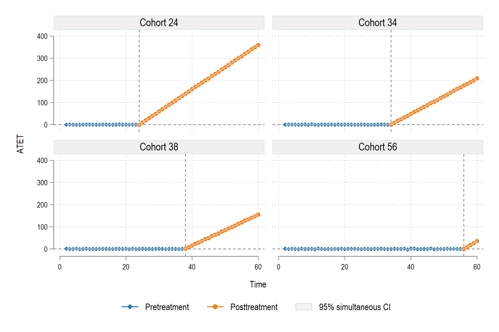
The command’s built-in graph option gives us:
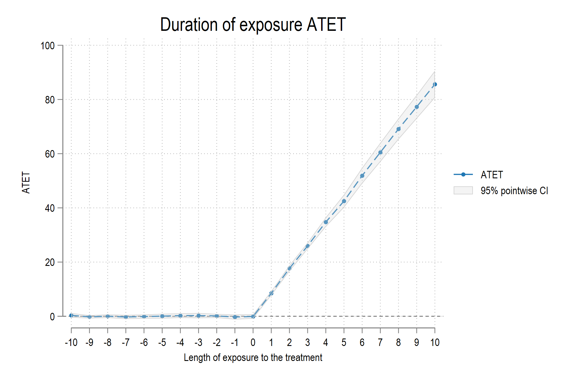
estat aggregation, dynamic(-10(1)10) graph