did_multiplegt (Chaisemartin and D’Haultfœuille 2020, 2021)
Note
To estimate event-study/dynamic effects, we strongly recommend using the much faster did_multiplegt_dyn command.
In addition to that, did_multiplegt_dyn offers more options than did_multiplegt, among which:
- normalized: estimation of the normalized dynamic effects (de Chaisemartin & D’Haultfoeuille, 2024);
- predict_het: built-in treatment effect heterogeneity analysis;
- design and date_first_switch: post-estimation options to analyze the design and timing of the treatment;
- by and by_path: estimating dynamic effects within levels of a group-level variable or within treatment paths;
- trends_lin: built-in group-specific linear trends.
Lastly, as of the last release, did_multiplegt_dyn also includes two user-requested features:
- only_never_switchers: restricting the estimators from de Chaisemartin & D’Haultfoeuille (2024) to only compare switchers and never-switchers;
- integration with esttab: here a quick tutorial.
Table of contents
Installation and options
ssc install did_multiplegt, replace
Take a look at the help file:
help did_multiplegt
Test the command
Please make sure that you generate the data using the script given here
Let’s try the basic did_multiplegt command:
did_multiplegt Y id t D, robust_dynamic dynamic(10) placebo(10) breps(20) cluster(id) seed(0)
and we get this output:
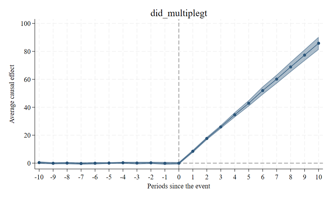
DID estimators of the instantaneous treatment effect, of dynamic treatment effects if the dynamic option is used,
and of placebo tests of the parallel trends assumption if the placebo option is used.
The estimators are robust to heterogeneous effects, and to dynamic effects if the robust_dynamic option is used.

             |  Estimate         SE      LB CI      UB CI          N  Switchers
-------------+-----------------------------------------------------------------
    Effect_0 | -.0608394   .3777101  -.8011512   .6794724         78         23
    Effect_1 |   8.49767    .371304   7.769914   9.225426         78         23
    Effect_2 |  17.64773   .4621524   16.74191   18.55355         78         23
    Effect_3 |   25.9377   .6017678   24.75823   27.11716         78         23
    Effect_4 |  34.62362   .9410695   32.77913   36.46812         75         23
    Effect_5 |  42.85682    1.30207   40.30476   45.40888         64         19
    Effect_6 |  51.93103   1.587562   48.81941   55.04265         64         19
    Effect_7 |  60.13327   1.959996   56.29168   63.97486         64         19
    Effect_8 |  68.82446   2.144383   64.62147   73.02745         64         19
    Effect_9 |  77.30792    2.51719   72.37423   82.24161         64         19
   Effect_10 |  85.78878   2.878414   80.14709   91.43047         55         19
     Average |  40.79851   1.198362   38.44972    43.1473        762        229
   Placebo_1 |  .1308918   .5623093  -.9712345   1.233018         78         23
   Placebo_2 | -.0635463   .3870331  -.8221312   .6950386         78         23
   Placebo_3 | -.1275425   .4243438  -.9592563   .7041713         78         23
   Placebo_4 | -.3848304   .3591436  -1.088752   .3190911         78         23
   Placebo_5 | -.4583827    .294038  -1.034697   .1179317         75         23
   Placebo_6 | -.1875761   .3982451  -.9681365   .5929843         64         19
   Placebo_7 |  .1194069   .4310281  -.7254083   .9642221         64         19
   Placebo_8 |  .0628537   .4707887   -.859892   .9855995         64         19
   Placebo_9 | -.1943704   .4800074  -1.135185    .746444         64         19
  Placebo_10 | -.2936845   .4425423  -1.161067   .5736984         64         19
The command also produces by default an event-study graph, unless the firstdiff_placebo option is specified: in that case, we do not recommend putting together first-difference placebos and long-difference event-study estimates on the same event-study graph.
We can also plot the results using the event_plot (ssc install event_plot, replace) command as follows:
event_plot e(estimates)#e(variances), default_look ///
	graph_opt(xtitle("Periods since the event") ytitle("Average causal effect") ///
	title("did_multiplegt") xlabel(-10(1)10)) stub_lag(Effect_#) stub_lead(Placebo_#) together
and we get this figure: