did_imputation
Table of contents
Notes
- Based on: Borusyak, Jaravel, Spiess 2021. Revisiting Event Study Designs: Robust and Efficient Estimation that was last revised on 16 Jan 2024 (v5).
- Program version (if available): November 22, 2023
- Last checked: Nov 2024
Installation
ssc install did_imputation, replace
Take a look at the help file:
help did_imputation
Test the command
Please make sure that you generate the data using the script given here
Let’s try the basic did_imputation command with 10 leads and lags:
did_imputation Y i t first_treat, horizons(0/10) pretrend(10) minn(0)
which gives us:
                                                         Number of obs = 1,438
------------------------------------------------------------------------------
           Y | Coefficient  Std. err.      z    P>|z|     [95% conf. interval]
-------------+----------------------------------------------------------------
        tau0 |   .0787163   .2677837     0.29   0.769      -.44613    .6035626
        tau1 |   8.637227   .2815466    30.68   0.000     8.085406    9.189048
        tau2 |   17.78728   .2329168    76.37   0.000     17.33078    18.24379
        tau3 |   26.07725   .2293303   113.71   0.000     25.62777    26.52673
        tau4 |   34.76562   .2815757   123.47   0.000     34.21374     35.3175
        tau5 |   42.93274   .2848896   150.70   0.000     42.37437    43.49111
        tau6 |   52.00695   .2787334   186.58   0.000     51.46064    52.55326
        tau7 |   60.20919   .2526519   238.31   0.000       59.714    60.70438
        tau8 |   68.90038   .2317813   297.26   0.000      68.4461    69.35466
        tau9 |   77.38383   .2652313   291.76   0.000     76.86399    77.90368
       tau10 |   85.83142    .309541   277.29   0.000     85.22473    86.43811
        pre1 |   .1206052   .2866341     0.42   0.674    -.4411872    .6823977
        pre2 |   .2116369   .3320804     0.64   0.524    -.4392287    .8625025
        pre3 |   .0601094   .2808867     0.21   0.831    -.4904184    .6106372
        pre4 |   .0568874   .2809316     0.20   0.840    -.4937285    .6075032
        pre5 |  -.2050823   .2642319    -0.78   0.438    -.7229672    .3128027
        pre6 |  -.3225205   .2343503    -1.38   0.169    -.7818387    .1367977
        pre7 |  -.2239894   .2511694    -0.89   0.373    -.7162724    .2682936
        pre8 |    .052194   .2243524     0.23   0.816    -.3875287    .4919166
        pre9 |   .0285485   .2358903     0.12   0.904    -.4337881     .490885
       pre10 |   .0962904   .2314293     0.42   0.677    -.3573028    .5498836
------------------------------------------------------------------------------
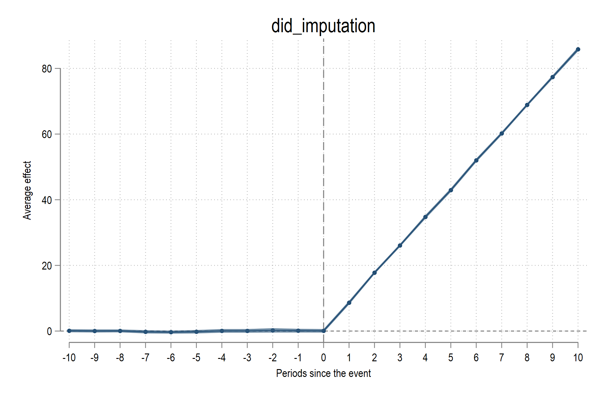
In order to plot the estimates we can use the event_plot (ssc install event_plot, replace) command as follows:
event_plot, default_look graph_opt(xtitle("Periods since the event") ytitle("Average effect") ///
	title("did_imputation") xlabel(-10(1)10)) stub_lag(tau#) stub_lead(pre#) together
And we get: