The Twoway Fixed Effects (TWFE) model
Table of contents
- The classic 2x2 DiD or the Twoway Fixed Effects Model (TWFE)
- The triple difference estimator (DDD)
- The generic TWFE functional form
- Stata Code
- Adding more time periods
- More units, same treatment time, different treatment effects
- More units, differential treatment time, different treatment effects
The classic 2x2 DiD or the Twoway Fixed Effects Model (TWFE)
incomplete
Let us start with the classic Twoway Fixed Effects (TWFE) model:
\[y_{it} = \beta_0 + \beta_1 Treat_i + \beta_2 Post_t + \beta_3 Treat_i Post_t + \epsilon_{it}\]The above two by two (2x2) model can be explained using the following table:
| Treatment = 0 | Treatment = 1 | Difference | |
|---|---|---|---|
| Post = 0 | \(\beta_0\) | \(\beta_0 + \beta_1\) | \(\beta_1\) |
| Post = 1 | \(\beta_0 + \beta_2\) | \(\beta_0 + \beta_1 + \beta_2 + \beta_3\) | \(\beta_1 + \beta_3\) |
| Difference | \(\beta_2\) | \(\beta_2 + \beta_3\) | \(\beta_3\) |
The triple difference estimator (DDD)
incomplete
The triple difference estimator essential takes two DDs, one with the target unit of analysis with a treated and an untreated group. This is compared to another similar group in the pre and post-treatment period. Fo effectively there are two treatments. One where an actual treatment on the desired group is tested, and a placebo comparison group, on which the same intervention is also applied.
\[y_{it} = \beta_0 + \beta_1 P_{i} + \beta_2 C_{j} + \beta_3 T_t + \beta_4 (P_i T_t) + \beta_5 (C_j T_t) + \beta_6 (P_i C_j) + \beta_7 (P_i C_j T_t) + \epsilon_{it}\]where we have 3x3 combinations: P = {0,1}, T={0,1}, C={0,1}. As is the case with the 2x2 DD, here the coefficient of interest is \(\beta_7\). This can also be broken down in a table form. But rather than create one big table, the results are usually presented for C = 0, or the main treatment group, and for C = 1, or the main comparison group. The difference between the two boils down to \(\beta_7\). Let’s see this here:
Main group (\(C = 0\)):
| T = 0 | T = 1 | Difference | |
|---|---|---|---|
| P = 0 | \(\beta_0\) | \(\beta_0 + \beta_3\) | \(\beta_3\) |
| P = 1 | \(\beta_0 + \beta_1\) | \(\beta_0 + \beta_1 + \beta_3 + \beta_4\) | \(\beta_3 + \beta_4\) |
| Difference | \(\beta_1\) | \(\beta_1 + \beta_4\) | \(\beta_4\) |
Comparison group (\(C = 1\)):
| T = 0 | T = 1 | Difference | |
|---|---|---|---|
| P = 0 | \(\beta_0 + \beta_2\) | \(\beta_0 + \beta_2 + \beta_3 + \beta_5\) | \(\beta_3 + \beta_5\) |
| P = 1 | \(\beta_0 + \beta_1 + \beta_2 + \beta_6\) | \(\beta_0 + \beta_1 + \beta_2 + \beta_3 + \beta_4 + \beta_5 + \beta_6 + \beta_7\) | \(\beta_3 + \beta_4 + \beta_5 + \beta_7\) |
| Difference | \(\beta_1 + \beta_6\) | \(\beta_1 + \beta_4 + \beta_6 + \beta_7\) | \(\beta_4 + \beta_7\) |
Let’s take the difference between the two matrices or (C = 1) - (C = 0):
| T = 0 | T = 1 | Difference | |
|---|---|---|---|
| P = 0 | \(\beta_2\) | \(\beta_2 + \beta_5\) | \(\beta_5\) |
| P = 1 | \(\beta_2 + \beta_6\) | \(\beta_2 + \beta_5 + \beta_6 + \beta_7\) | \(\beta_5 + \beta_7\) |
| Difference | \(\beta_6\) | \(\beta_6 + \beta_7\) | \(\beta_7\) |
where we end up with the main difference of \(\beta_7\). Note that this table logic is also far simpler than having a long list of expectations defined for each combination.
The generic TWFE functional form
incomplete
If we have multiple time periods and treatment units, the classic 2x2 DiD can be extended to the following generic functional form:
\[y_{it} = \alpha_{i} + \alpha_t + \beta^{TWFE} D_{it} + \epsilon_{it}\]Stata Code
Let us generate a simple 2x2 example in Stata. First step define the panel structure. Since it is a 2x2, we just need two units and two time periods:
clear
local units = 2
local start = 1
local end   = 2

local time = `end' - `start' + 1
local obsv = `units' * `time'
set obs `obsv'

egen id	   = seq(), b(`time')
egen t 	   = seq(), f(`start') t(`end')

sort id t
xtset id t

lab var id "Panel variable"
lab var t  "Time  variable"
Next we define the treatment group and a generic TWFE model without adding any variation or error terms:
gen D = id==2 & t==2

gen btrue = cond(D==1, 2, 0)
	gen Y = id + 3*t + btrue*D
According to the last line, the treatment effect should have an impact of 3 units on Y in the post group. We can check this by plotting the data:
lab de prepost 1 "Pre" 2 "Post"
lab val t prepost

twoway ///
	(connected Y t if id==1) ///
	(connected Y t if id==2) ///
		,	///
		legend(order(1 "id=1" 2 "id=2")) ///
		xlabel(1 2, valuelabel) ylabel(4(1)10)
which gives us:
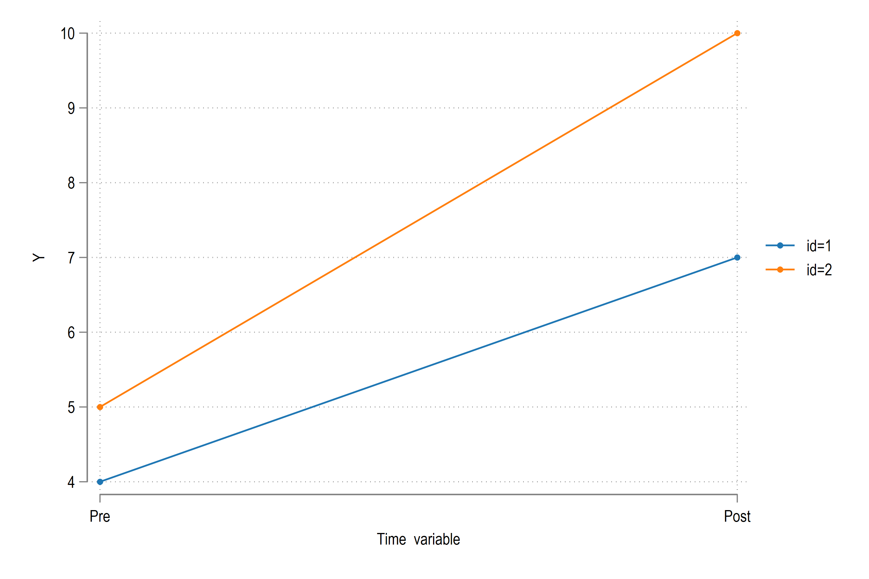
where we can see that the difference between the blue and the orange line is 3 in the post period, and 1 in the pre-period, making it a net gain of 2 units. Which also equals the treatment amount we specified.
We can also recover this from a simple panel regression:
xtset id t
xtreg Y D t, fe
In the regression, you will see that the coefficient of D, \(\beta^{TWFE}\) = 2, as expected. An alternative way of doing this is to use the reghdfe package, which we will also call in later examples:
reghdfe Y D, absorb(id t)
which again gives us the same result for the D coefficient.
Adding more time periods
Now that we are comfortable with the 2x2 example, let’s add more time periods. How about 10 per unit:
clear
local units = 2
local start = 1
local end 	= 10

local time = `end' - `start' + 1
local obsv = `units' * `time'
set obs `obsv'

egen id	   = seq(), b(`time')
egen t 	   = seq(), f(`start') t(`end')

sort  id t
xtset id t

lab var id "Panel variable"
lab var t  "Time  variable"
And we just do a simple treatment where id=2 increases by 3 units at time period 5 and stays there:
gen D = id==2 & t>=5
lab var D "Treated"

gen btrue = cond(D==1, 3, 0)

gen Y = id + t +  btrue*D
lab var Y "Outcome variable"
We can also visualize this as follows:
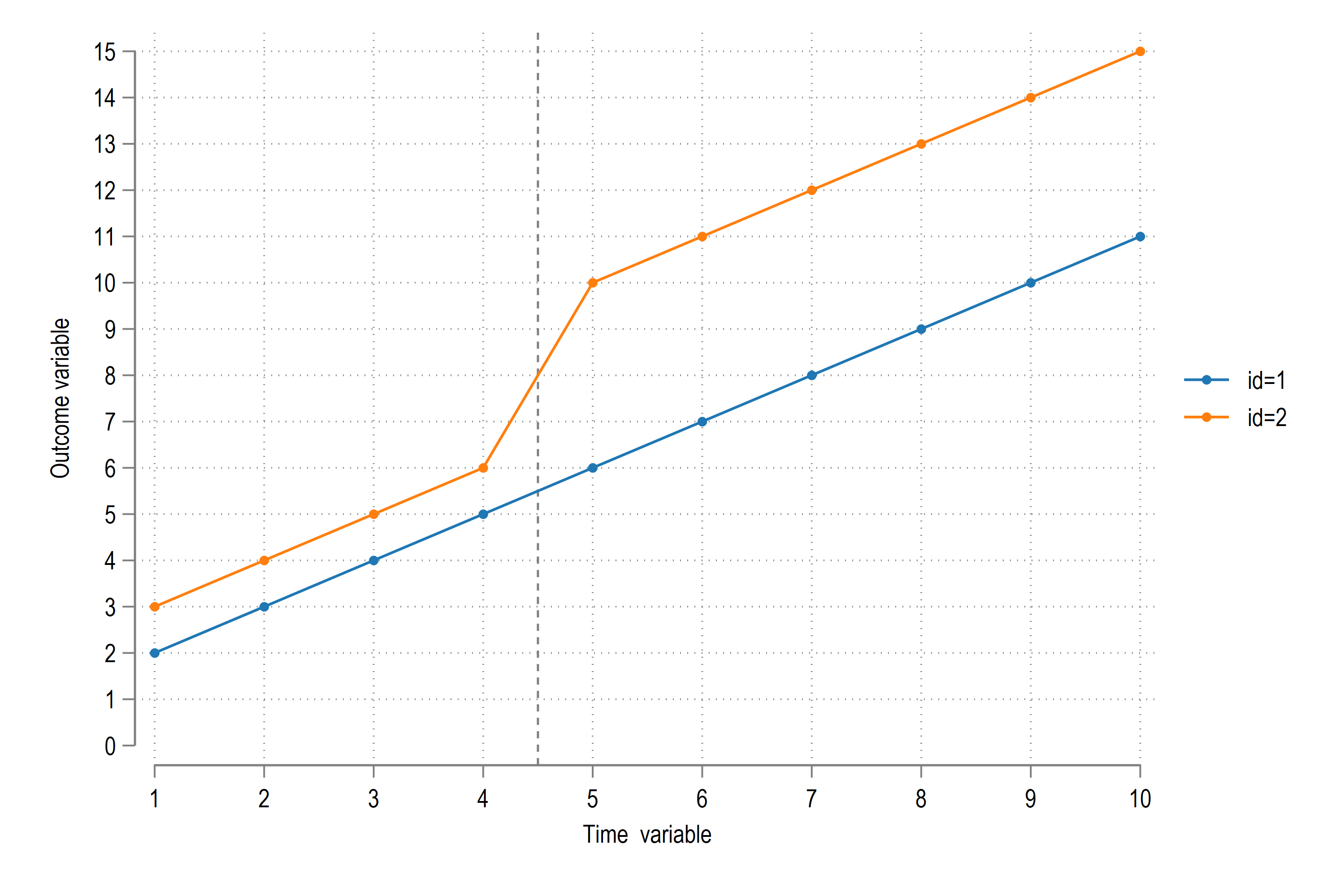
and we can also run the Stata code:
xtreg Y D t, fe
reghdfe Y D, absorb(id t)
The xtreg option shows that \(t\) on average increases by 1 unit, which is what we expect. The intercept equals 1.5, which is the average of the blue and orange lines if they are extrapolated to \(t = 0\) point. And \(\) \beta^{TWFE} \(= 3\), the true value of the intervention effect.
More units, same treatment time, different treatment effects
Let’s start with a very case where we have one control group, two treatment groups. The two T groups recieve treatment at the same time but with treatment intensities:
clear
local units = 3
local start = 1
local end 	= 10

local time = `end' - `start' + 1
local obsv = `units' * `time'
set obs `obsv'

egen id	   = seq(), b(`time')
egen t 	   = seq(), f(`start') t(`end')

lab var id "Panel variable"
lab var t  "Time  variable"

sort  id t
xtset id t


gen D = 0
replace D = 1 if id>=2 & t>=5
lab var D "Treated"

cap drop Y
gen Y = 0
replace Y = cond(D==1, 2, 0) if id==2
replace Y = cond(D==1, 4, 0) if id==3

lab var Y "Outcome variable"
and plot it:
twoway ///
	(connected Y t if id==1) ///
	(connected Y t if id==2) ///
	(connected Y t if id==3) ///
		,	///
		xline(4.5) ///
		xlabel(1(1)10) ///
		legend(order(1 "id=1" 2 "id=2" 3 "id=3"))
from which we get:
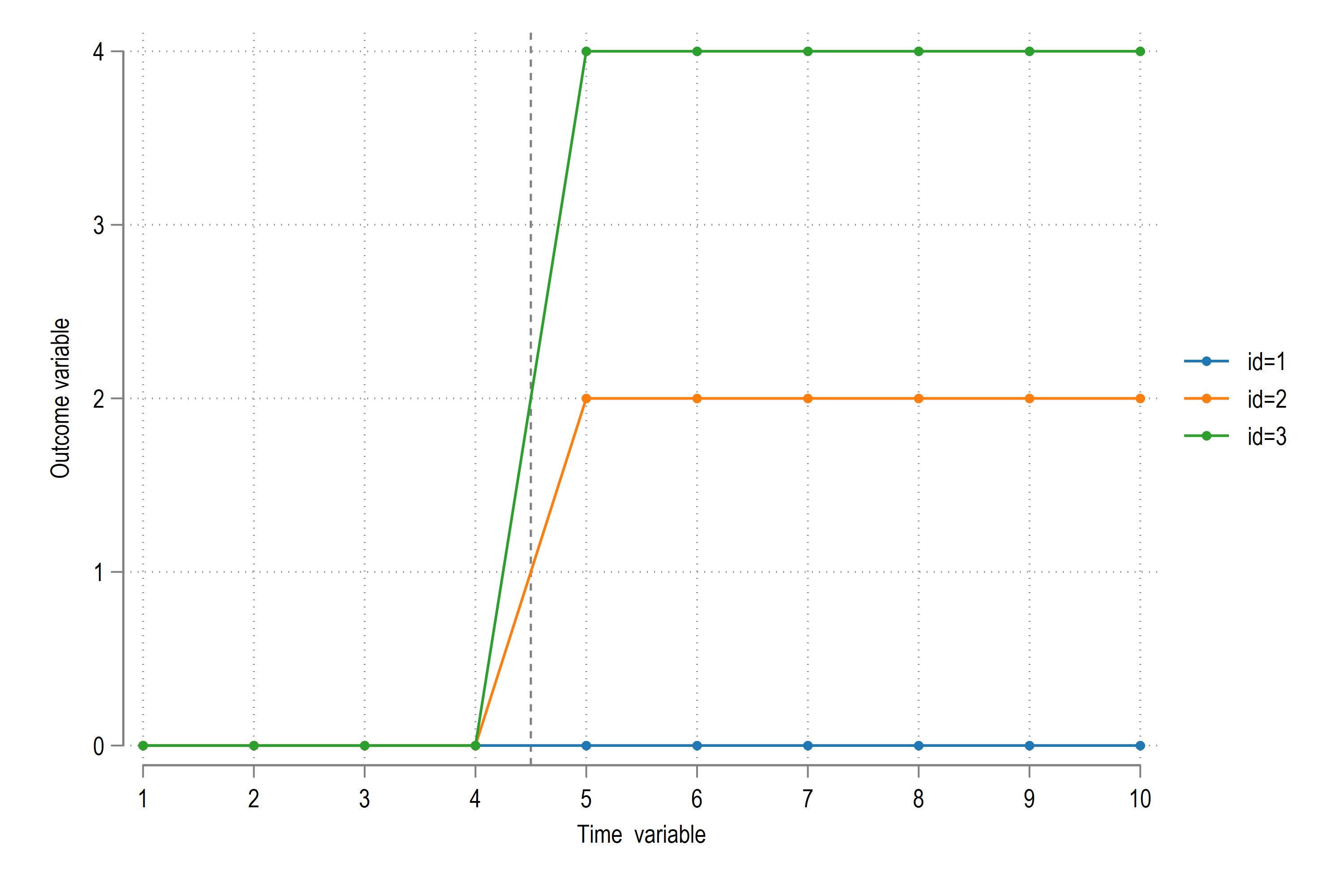
Here we can see that the post treatement has an average effect of 2 on id=2 and 4 on id=3. This implies that the ATT equals \(\beta^{TWFE}\)=3, which we can also check by recovering the coefficients:
xtreg Y D t, fe
While it is easy to check here the average treatment effect, since they are no time or panel fixed effects, we can basically visually see how the outcomes are changing. But if we add controls, it gets a bit more complicated. Let’s just generate the code in one go:
clear
local units = 3
local start = 1
local end 	= 10

local time = `end' - `start' + 1
local obsv = `units' * `time'
set obs `obsv'

egen id	   = seq(), b(`time')
egen t 	   = seq(), f(`start') t(`end')

sort  id t
xtset id t

lab var id "Panel variable"
lab var t  "Time  variable"

gen D = 0
replace D = 1 if id>=2 & t>=5
lab var D "Treated"

cap drop Y
gen Y = 0
replace Y = id + t + cond(D==1, 0, 0) if id==1
replace Y = id + t + cond(D==1, 2, 0) if id==2
replace Y = id + t + cond(D==1, 4, 0) if id==3

lab var Y "Outcome variable"

twoway ///
	(connected Y t if id==1) ///
	(connected Y t if id==2) ///
	(connected Y t if id==3) ///
		,	///
		xline(4.5) ///
		xlabel(1(1)10) ///
		legend(order(1 "id=1" 2 "id=2" 3 "id=3"))
From the earlier example, we know that the ATT equals \(\beta^{TWFE}\)=3, but from the graphs we can cannot see this so clearly. This is because we need to get rid of panel and id time trends. While we can also do this partialling out by hand (but we won’t), we can use our regression specification:
xtreg Y D t, fe
which gives the ATT=3, which is the average of the two treatment variables.
Here, I would like to add that parallel trend assumptions are controlled for in the above regression specification. If these are not accounted for, then we basically end up with the wrong ATTs. We can see the D coefficients in the follow regressions:
reg Y D				// not controlling for any effects
reg Y D i.t			// only time fixed effects
reg Y D i.id		// only panel fixed effects
reg Y D i.t i.id	// panel and time fixed effects (correct!)
More units, differential treatment time, different treatment effects
Now let’s move on to the final part: treatments with differential timings. Here we again generate a dummy dataset but get rid of panel and time fixed effects for now. As we have seen above, the regressions isolate the panel fixed effects and we recover the coefficient of interest \(\beta^{TWFE}\).
clear
local units = 3
local start = 1
local end 	= 10

local time = `end' - `start' + 1
local obsv = `units' * `time'
set obs `obsv'

egen id	   = seq(), b(`time')
egen t 	   = seq(), f(`start') t(`end')

sort  id t
xtset id t

lab var id "Panel variable"
lab var t  "Time  variable"

gen D = 0
replace D = 1 if id==2 & t>=5
replace D = 1 if id==3 & t>=8
lab var D "Treated"

gen Y = 0
replace Y = D * 2 if id==2 & t>=5
replace Y = D * 4 if id==3 & t>=8

lab var Y "Outcome variable"


twoway ///
	(connected Y t if id==1) ///
	(connected Y t if id==2) ///
	(connected Y t if id==3) ///
		,	///
		xline(4.5 7.5) ///
		xlabel(1(1)10) ///
		legend(order(1 "id=1" 2 "id=2" 3 "id=3"))
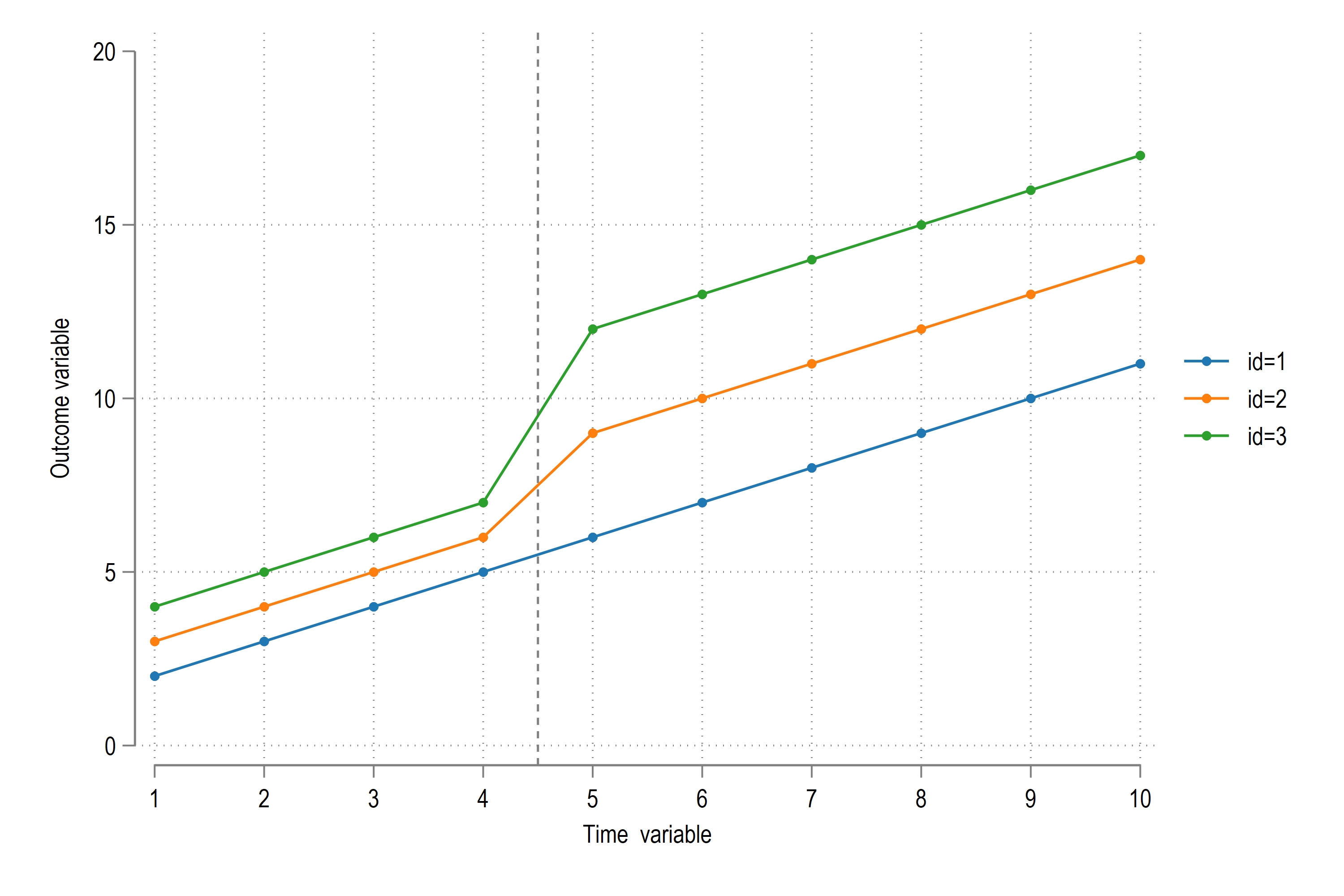
which gives us this figure:
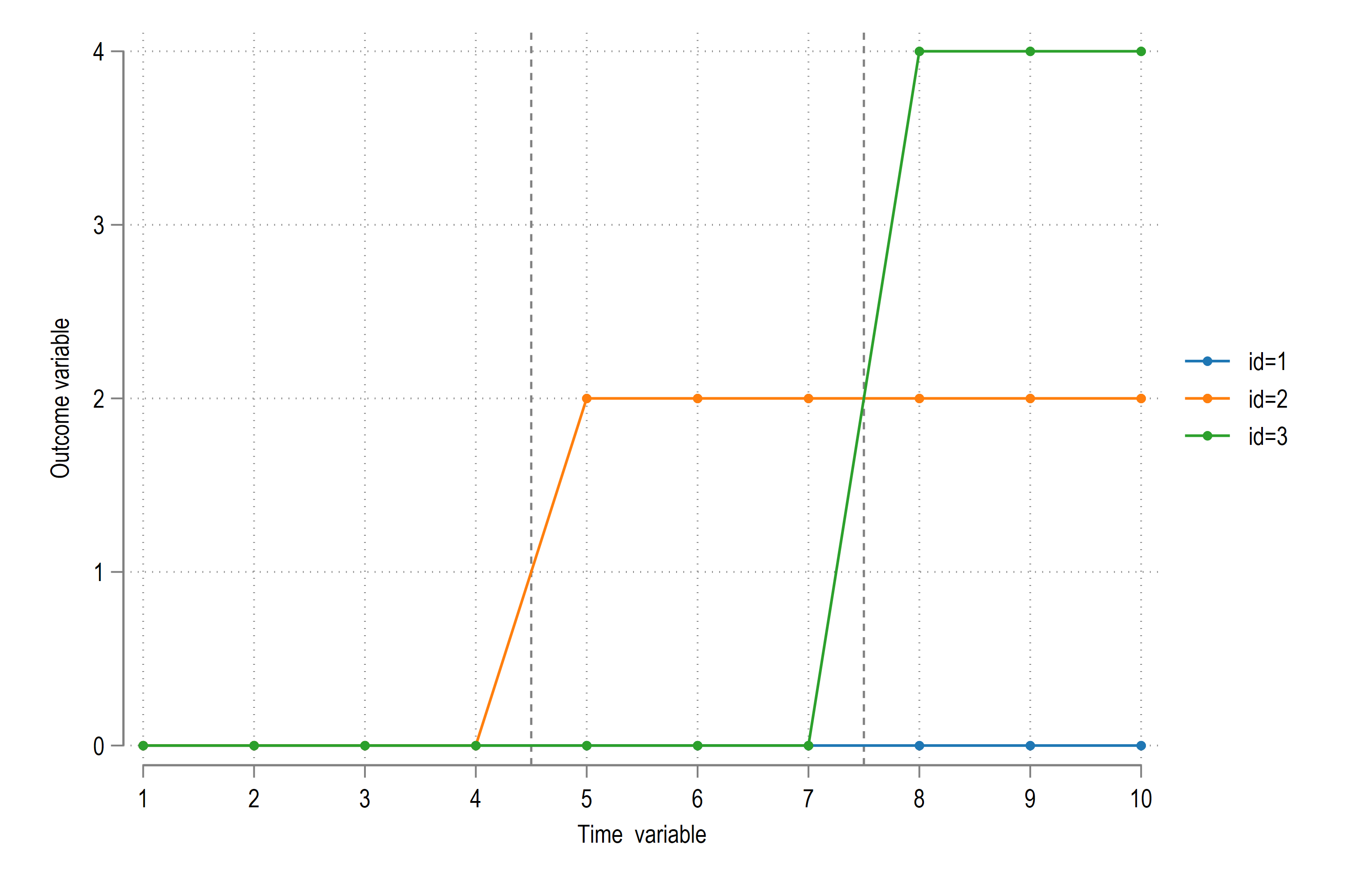
The figure shows that the group id=2 gets the intervention at t=5 and stays treated, while the group id=3 gets the intervention at t=8 and stays treated. So what is the ATT here?
Unlike the previous examples, were we could derive the ATT, just by looking at the graph, it is not so trivial here. Even though there are no time and panel fixed effects, differentials in treatment time does make changes over panel and time relevant. Without going into the maths, to recover the actual ATT, we need to average out time and panel effects for treated and non-treated observations.
We can do these regressions to see the outcomes:
reg Y D				// not controlling for any effects
reg Y D i.t			// only time fixed effects
reg Y D i.id		// only panel fixed effects
reg Y D i.t i.id	// panel and time fixed effects (correct!)
The last regression gives us the correct ATT which is \(\beta^{TWFE}\) = 2.91. This is, in fact, the average increase in \(y_{it}\) after averaging out for panel and time variables.
We can also recover this using the standard commands:
xtreg Y D i.t, fe
reghdfe Y D, absorb(id t)
which gives us the same answer of \(\beta^{TWFE}\) = 2.91.
Let’s think about this number for a bit. We have two treatments happening at different times with different treatment effects. Therefore the definition of pre and post is not clear anymore. Neither is untreated versus treated. if we look at the interval \(5\leq t < 8\), only id=2 is changing, and the other two variables are constant. But in the last interval where \(t \geq 8\), then only id=3 is showing a change, while the other two panel variables are constant in this interval (even through id=2 is treated here).
It is these combinations that are unraveled in the section on Bacon decomposition, which is why, it is important understand the decomposition carefully.