did_multiplegt (Chaisemartin and D’Haultfœuille 2020, 2021)
Note
To estimate event-study/dynamic effects, we strongly recommend using the much faster did_multiplegt_dyn command.
In addition to that, did_multiplegt_dyn offers more options than did_multiplegt, among which:
- normalized: estimation of the normalized dynamic effects (de Chaisemartin & D’Haultfoeuille, 2024);
- predict_het: built-in treatment effect heterogeneity analysis;
- design and date_first_switch: post-estimation options to analyze the design and timing of the treatment;
- by and by_path: estimating dynamic effects within levels of a group-level variable or within treatment paths;
- trends_lin: built-in group-specific linear trends.
Lastly, as of the last release, did_multiplegt_dyn also includes several user-requested features:
- only_never_switchers: restricting the estimators from de Chaisemartin & D’Haultfoeuille (2024) to only compare switchers and never-switchers;
- the output of did_multiplegt_dyn can be assigned (ex:
did <- did_multiplegt_dyn(df, Y, G, T, D)) as a list with did_multiplegt_dyn class; - custom class allows for built-in customized print() and summary() methods;
- the displayed output can be retrieved in full from the assigned object by simply browsing the list;
- integration with ggplot2: the assigned output will always contain a ggplot object for the event-study graph.
Table of contents
Introduction
The DIDmultiplegt package implements the estimation procedure proposed by de Chaisemartin and D’Haultfœuille (2020) (henceforth dCDH20). A key virtue of dCDH20 is that is one of the most flexible DiD estimators currently available. It allows for treatment switching (units can move in and out of treatment status) in addition to time-varying, heterogeneous treatment effects.
On the downside, the command is the slowest of the available DiD estimators by
some distance. This partly has to do with the fact that calculating standard
errors require bootstrap replications, and adding additional options multiplies
the number of estimation calculations in the background. On the other hand, the
R implementation does support parallelization—at least on Linux and
Mac—and appears to be quite a bit faster than the Stata equivalent. But
there is still no display or progress bar while the command is running, so it is
hard to track estimation times (which may take several minutes even for small
datasets). Moreover, the package does not provide standard methods like
summary and print that one would typicaly use to interogate a model object
in R. So, it does suffer from a lack of usability. I’ll try to how you some ways
to overcome this issue in the examples that follow.
Installation and options
The package can be installed from CRAN
install.packages("DIDmultiplegt") # Install (only need to run once or when updating)
library("DIDmultiplegt") # Load the package into memory (required each new session)
The main workhorse function of the package is did_multiplegt(), which in its
simplest form looks like:
did_multiplegt(df, Y, G, T, D, ...)
where
| Variable | Description |
|---|---|
| df | dataset |
| Y | outcome variable |
| G | group variable |
| T | time variable |
| D | treatment dummy variable (=1 if treated) |
| … | Additional arguments |
Again, a key strength of did_multiplegt() is that allows for very flexible
estimation strategies and requirements. There are a variety of additional
function arguments aimed at supporting or invoking these flexibilities. We’ll
cover a few of the most important ones below, but you can take a look at the
helpfile (?did_multiplegt) for more detailed information.
Dataset
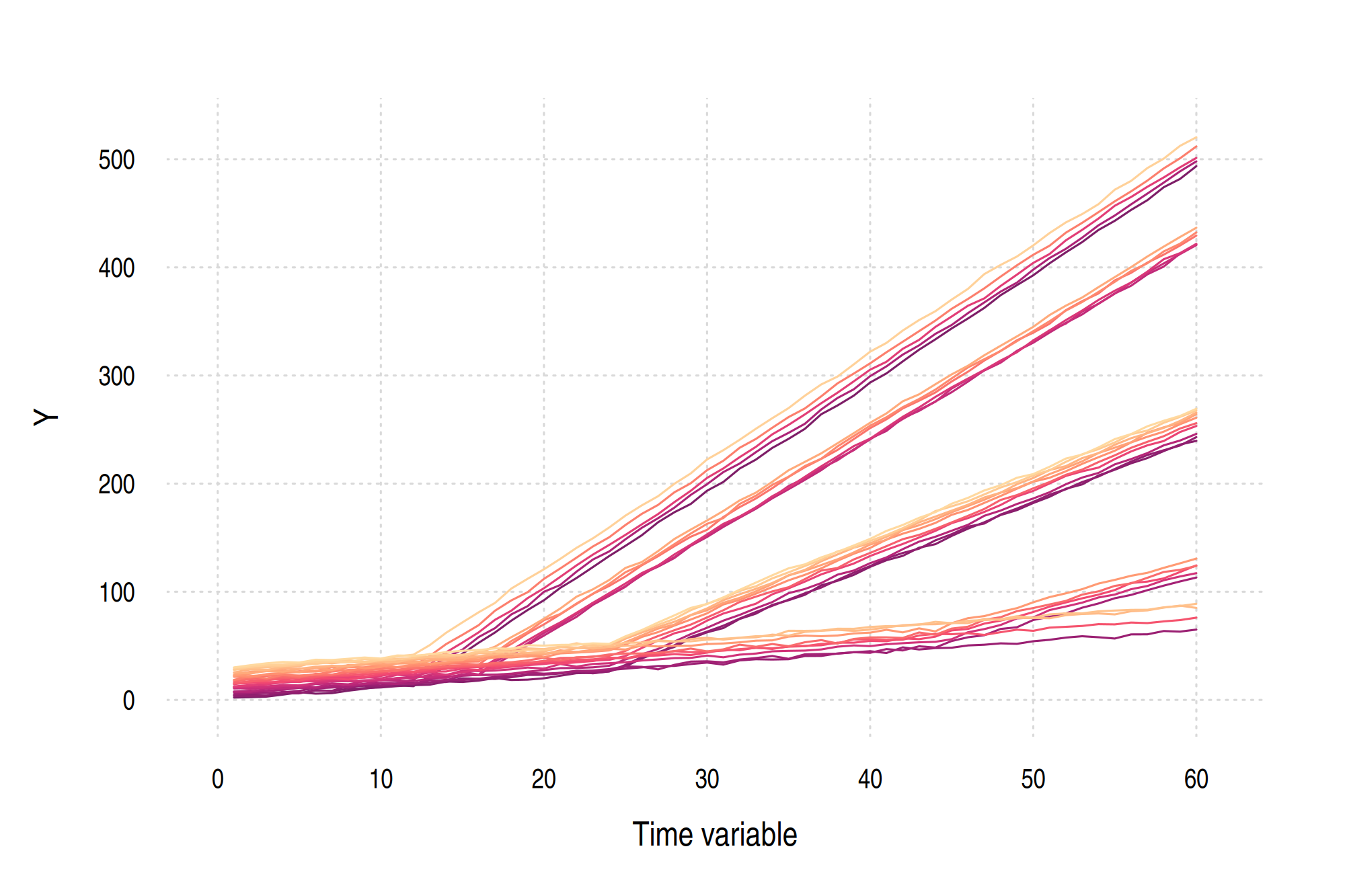
To demonstrate the package in action, we’ll use the fake dataset generated in the shared setup block here. Here’s a reminder of what the data look like.
head(dat)
#>   time id        y rel_time treat first_treat
#> 1    1  1 2.158289      -11 FALSE          12
#> 2    2  1 2.498052      -10 FALSE          12
#> 3    3  1 3.034077       -9 FALSE          12
#> 4    4  1 4.886266       -8 FALSE          12
#> 5    5  1 7.085950       -7 FALSE          12
#> 6    6  1 5.788352       -6 FALSE          12
Or, in graph form.
Test the package
Remember to load the package (if you haven’t already).
library(DIDmultiplegt)
Let’s try the basic did_multiplegt() command:
did_multiplegt(df = dat, Y = "y", G = "id", T = "time", D = "treat")
#> $effect
#>  treatment
#> -0.4571712
#>
#> $N_effect
#> [1] 83
#>
#> $N_switchers_effect
#> [1] 26
That completes pretty quickly (a couple of seconds), but isn’t particularly information rich. It’s just a point estimate of the instantaneous treatment effect (i.e. the time period when switchers switch). So let’s try a more realistic use-case by invoking additional function arguments…
To start, note that we can get bootstrapped standard errors by invoking the
breps argument. We’ll also go ahead and estimate an actual event study with 10
pre-treatment leads and 10 post-treatment lags (somewhat confusingly in the
dCDH20 framework referred to as placebo and dynamic periods, respectively).
This time, I’ll also save the resulting model object, although note that it will
take significantly longer to estimate. (Over 6 minutes on my laptop, despite
invoking parallelization to use all 12 available threads.)
mod_dCDH20 = did_multiplegt(
  dat, 'y', 'id', 'time', 'treat', # original regression params
  dynamic   = 10,                  # no. of post-treatment periods
  placebo   = 10,                  # no. of pre-treatment periods
  brep      = 20,                  # no. of bootstraps (required for SEs)
  cluster   = 'id',                # variable to cluster SEs on
  parallel  = TRUE                 # run the bootstraps in parallel
  )
Running the above command will automically yield the following event study plot.
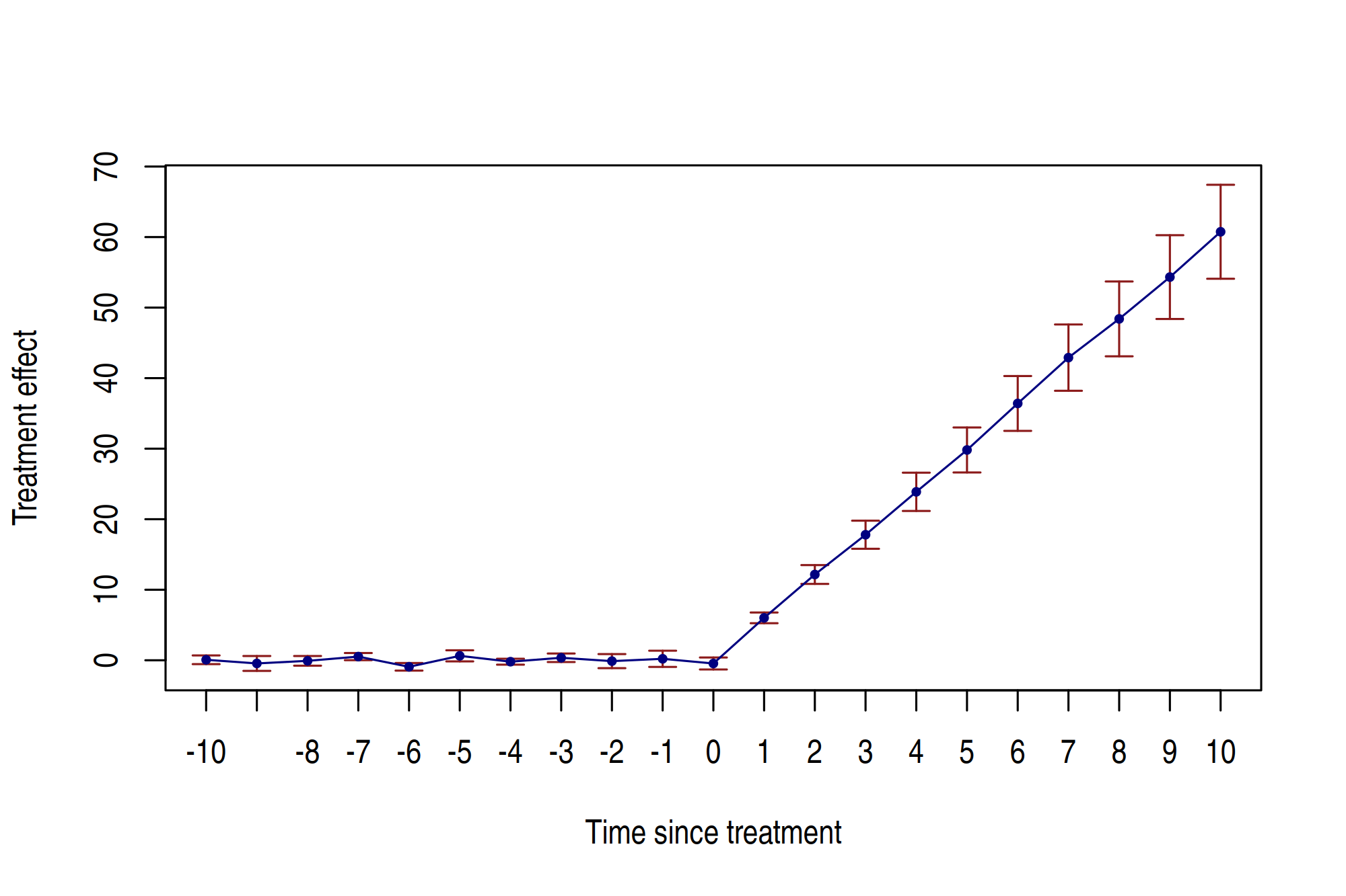
While the above plot is pretty nice—and can be exported/saved for future
use— the truth is that our return mod_dCDH20 object is not particularly
user-friendly. It’s just a list and lacks an explicit model class. As such, it
doesn’t provide the standard set of convenience methods that we would expect for
model objects in R, e.g. summary or print.
head(mod_dCDH20)
#> $placebo_10
#> [1] 0.06805525
#>
#> $se_placebo_10
#> [1] 0.3151775
#>
#> $N_placebo_10
#> [1] 83
#>
#> $placebo_9
#> [1] -0.4496167
#>
#> $se_placebo_9
#> [1] 0.5380869
#>
#> $N_placebo_9
#> [1] 83
You can follow this
issue to see when
some standard methods will be added to the package. In the meantime, here’s a
quick function for converting the did_multiplegt objects into a “tidy” data
frame, a la broom conventions.
# install.packages("broom")
library(broom)

# Create a tidier for "multiplegt" objects
tidy.did_multiplegt = function(x, level = 0.95) {
  ests = x[grepl("^placebo_|^effect|^dynamic_", names(x))]
  ret = data.frame(
    term      = names(ests),
    estimate  = as.numeric(ests),
    std.error = as.numeric(x[grepl("^se_placebo|^se_effect|^se_dynamic", names(x))]),
    N         = as.numeric(x[grepl("^N_placebo|^N_effect|^N_dynamic", names(x))])
    ) |>
    # For CIs we'll assume standard normal distribution
    within({
      conf.low  = estimate - std.error*(qnorm(1-(1-level)/2))
      conf.high = estimate + std.error*(qnorm(1-(1-level)/2))
      })
  return(ret)
}
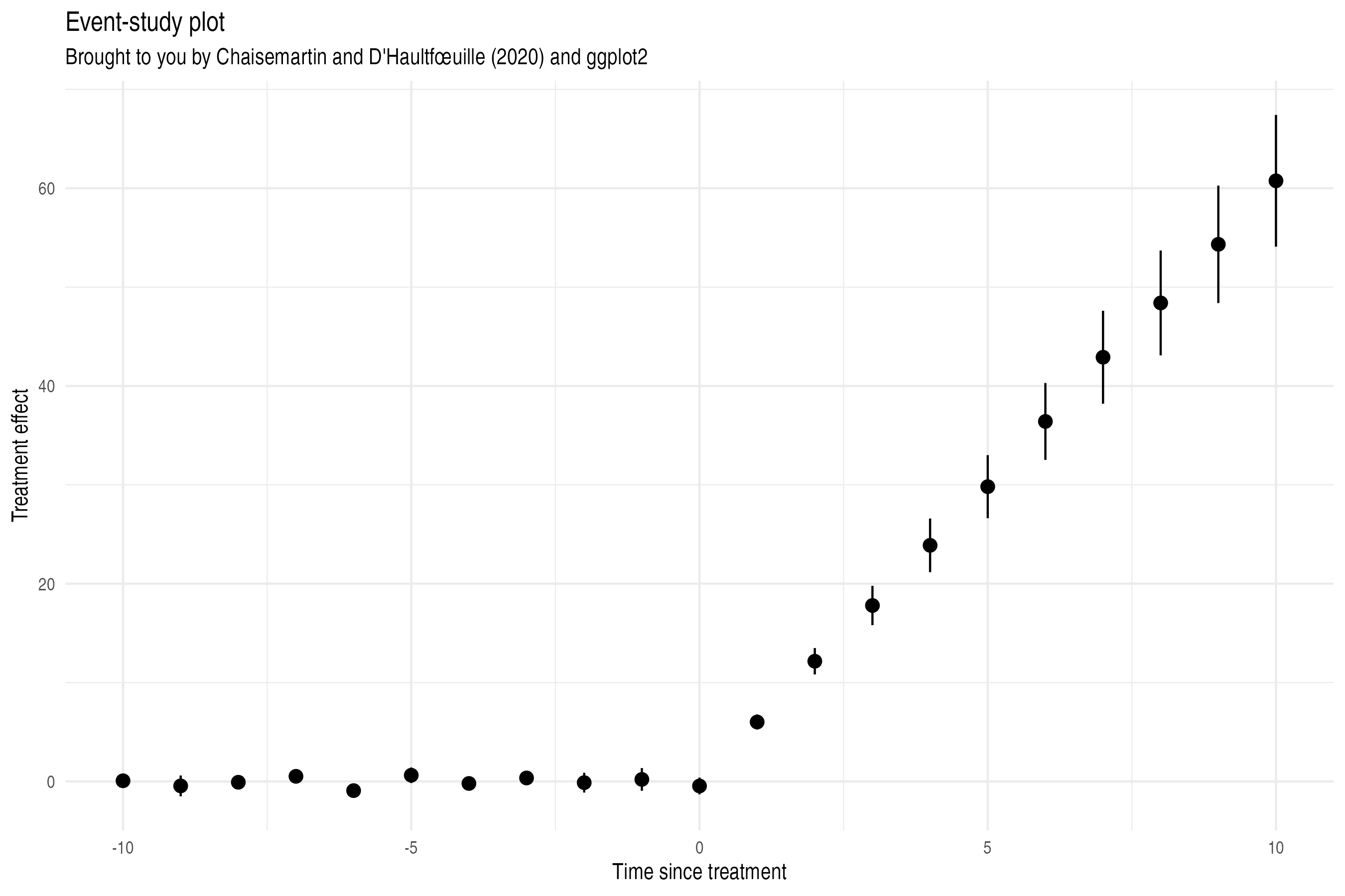
Now we can use our little function to view the estimation results in much
friendlier data frame format. In turn, this data frame makes it easy to
constuct your own (bespoke) event-study plots using either the base R plot()
function or ggplot2.
tidy_dCDH20 = tidy(mod_dCDH20)
tidy_dCDH20
#>          term    estimate std.error  N  conf.high    conf.low
#> 1  placebo_10  0.06805525 0.3151775 83  0.6857918 -0.54968129
#> 2   placebo_9 -0.44961673 0.5380869 83  0.6050142 -1.50424768
#> 3   placebo_8 -0.08261323 0.3500397 83  0.6034519 -0.76867836
#> 4   placebo_7  0.51945343 0.2586573 83  1.0264123  0.01249453
#> 5   placebo_6 -0.92753693 0.2747529 83 -0.3890312 -1.46604263
#> 6   placebo_5  0.62703000 0.4021329 83  1.4151960 -0.16113600
#> 7   placebo_4 -0.20311433 0.2146316 83  0.2175558 -0.62378446
#> 8   placebo_3  0.35268709 0.3082441 83  0.9568345 -0.25146028
#> 9   placebo_2 -0.12184467 0.5099217 83  0.8775835 -1.12127286
#> 10  placebo_1  0.20542543 0.5867543 83  1.3554428 -0.94459195
#> 11     effect -0.45717121 0.4331831 83  0.3918520 -1.30619441
#> 12  dynamic_1  6.01240948 0.3870975 83  6.7711067  5.25371223
#> 13  dynamic_2 12.15926002 0.6807289 83 13.4934641 10.82505594
#> 14  dynamic_3 17.79738274 1.0158897 83 19.7884900 15.80627550
#> 15  dynamic_4 23.88198369 1.3854778 77 26.5974703 21.16649703
#> 16  dynamic_5 29.81641003 1.6276905 77 33.0066249 26.62619521
#> 17  dynamic_6 36.41289963 1.9836774 77 40.3008360 32.52496330
#> 18  dynamic_7 42.90801358 2.3987287 77 47.6094354 38.20659181
#> 19  dynamic_8 48.40043286 2.7062129 67 53.7045128 43.09635296
#> 20  dynamic_9 54.32903314 3.0309359 67 60.2695583 48.38850799
#> 21 dynamic_10 60.75243562 3.3986148 67 67.4135983 54.09127299

# install.packages("ggplot2")
library(ggplot2)
theme_set(theme_minimal(base_family = "ArialNarrow")) # Optional

tidy_dCDH20 |>
  within({
    term = gsub("^placebo_", "-", term)
    term = gsub("^effect", "0", term)
    term = gsub("^dynamic_", "", term)
    term = as.integer(term)
    }) |>
  ggplot(aes(x = term, y = estimate, ymin = conf.low, ymax = conf.high)) +
  geom_pointrange() +
  labs(
    x = "Time to treatment", y = "Effect size", title = "Event-study plot",
    subtitle = "Brought to you by Chaisemartin and D'Haultfœuille (2020) and ggplot2"
    )
TO-DO: Check integration/complementarity with TwoWayFEWeights.