stackedev (Cengiz, Dube, Lindner, Zipperer 2019)
Table of contents
Introduction
The stackedev command is written by Joshua Bleiberg based on the Cengiz, Dube, Lindner, Zipperer 2019 QJE paper The effect of minimum wages on low-wage jobs.
The command is currently under active development so options might change around.
Installation and options
Install the command from SSC:
ssc install stackedev, replace
Take a look at the help file:
help stackedev
Test the command
Let’s run the basic stackedev
command:
stackedev Y F_* L_* ref, cohort(first_treat) time(t) never_treat(no_treat) unit_fe(id) clust_unit(id)
which will show this output:
**** Building Stack 24 ****
**** Building Stack 34 ****
**** Building Stack 38 ****
**** Building Stack 56 ****
**** Appending Stacks ****
**** Estimating Model with reghdfe ****
(MWFE estimator converged in 2 iterations)
warning: missing F statistic; dropped variables due to collinearity or too few clusters
note: ref omitted because of collinearity
HDFE Linear regression Number of obs = 3,060
Absorbing 2 HDFE groups F( 91, 49) = .
Statistics robust to heteroskedasticity Prob > F = .
R-squared = 0.9974
Adj R-squared = 0.9970
Within R-sq. = 0.9896
Number of clusters (unit_stack) = 50 Root MSE = 4.1332
(Std. err. adjusted for 50 clusters in unit_stack)
------------------------------------------------------------------------------
| Robust
Y | Coefficient std. err. t P>|t| [95% conf. interval]
-------------+----------------------------------------------------------------
F_2 | .2173356 .429718 0.51 0.615 -.6462151 1.080886
F_3 | .1386198 .4137917 0.33 0.739 -.6929257 .9701654
F_4 | -.0771335 .4251788 -0.18 0.857 -.9315624 .7772953
F_5 | -.3127445 .3628929 -0.86 0.393 -1.042005 .4165161
F_6 | -.4361147 .4095256 -1.06 0.292 -1.259087 .3868578
F_7 | -.3144571 .526613 -0.60 0.553 -1.372726 .7438113
F_8 | -.1044745 .4800377 -0.22 0.829 -1.069146 .8601974
F_9 | -.1156501 .4238786 -0.27 0.786 -.9674661 .7361659
F_10 | .1485313 .4001261 0.37 0.712 -.6555522 .9526148
F_11 | -.2473913 .47278 -0.52 0.603 -1.197478 .7026957
F_12 | -.1452927 .4785819 -0.30 0.763 -1.107039 .8164536
F_13 | .1286208 .4821393 0.27 0.791 -.8402744 1.097516
F_14 | .1440072 .3947098 0.36 0.717 -.6491919 .9372063
F_15 | .3114543 .476962 0.65 0.517 -.6470368 1.269945
F_16 | .1721978 .5333658 0.32 0.748 -.8996409 1.244037
F_17 | -.7585561 .3663682 -2.07 0.044 -1.494801 -.0223118
F_18 | .0699152 .5175897 0.14 0.893 -.9702202 1.110051
F_19 | -.3875619 .2815699 -1.38 0.175 -.9533978 .178274
F_20 | .0638705 .4198326 0.15 0.880 -.7798146 .9075557
F_21 | .035372 .4097576 0.09 0.932 -.7880668 .8588108
F_22 | -.5763502 .4471311 -1.29 0.203 -1.474894 .3221933
F_23 | .1005642 .3572709 0.28 0.780 -.6173985 .818527
F_24 | 4.715301 .9921569 4.75 0.000 2.721487 6.709115
F_25 | 3.848972 .9570067 4.02 0.000 1.925795 5.772149
F_26 | 3.885843 .9759061 3.98 0.000 1.924686 5.846999
F_27 | 3.665572 .9574264 3.83 0.000 1.741551 5.589592
F_28 | 3.629329 .9877625 3.67 0.001 1.644346 5.614312
F_29 | 4.376366 .9749251 4.49 0.000 2.41718 6.335551
F_30 | 4.38623 .9937478 4.41 0.000 2.389219 6.383241
F_31 | 3.95357 .9964798 3.97 0.000 1.951069 5.956071
F_32 | 4.131159 .9566808 4.32 0.000 2.208637 6.053681
F_33 | 4.421442 .9615812 4.60 0.000 2.489073 6.353812
F_34 | 3.870751 1.112861 3.48 0.001 1.634373 6.10713
F_35 | 3.975567 1.073438 3.70 0.001 1.818414 6.132721
F_36 | 3.999014 1.177784 3.40 0.001 1.632169 6.36586
F_37 | 3.909786 .9581247 4.08 0.000 1.984363 5.83521
F_38 | .9388715 .8728544 1.08 0.287 -.8151952 2.692938
F_39 | 1.211486 .7498948 1.62 0.113 -.2954839 2.718456
F_40 | 1.025343 .8874642 1.16 0.254 -.7580827 2.80877
F_41 | 1.526626 .606473 2.52 0.015 .3078726 2.745379
F_42 | 1.434986 .8133947 1.76 0.084 -.199592 3.069564
F_43 | 2.300906 .5985228 3.84 0.000 1.09813 3.503683
F_44 | 2.221324 .7714936 2.88 0.006 .6709491 3.771698
F_45 | .4473907 .6918146 0.65 0.521 -.9428628 1.837644
F_46 | 1.606906 .5320911 3.02 0.004 .537629 2.676183
F_47 | 1.220467 .99843 1.22 0.227 -.7859536 3.226887
F_48 | 1.43739 .6826501 2.11 0.040 .0655537 2.809227
F_49 | 1.691145 .6603621 2.56 0.014 .3640975 3.018192
F_50 | .5937526 .5885007 1.01 0.318 -.5888838 1.776389
F_51 | 1.543893 .5838527 2.64 0.011 .370597 2.717189
F_52 | 1.815931 .5872599 3.09 0.003 .635788 2.996074
F_53 | 1.176133 .679497 1.73 0.090 -.1893669 2.541634
F_54 | 2.117263 .9070423 2.33 0.024 .2944931 3.940032
F_55 | 1.314801 .5422668 2.42 0.019 .2250752 2.404527
L_0 | .0100481 .498877 0.02 0.984 -.9924828 1.012579
L_1 | 8.452976 .4244544 19.91 0.000 7.600003 9.305949
L_2 | 17.61775 .4799071 36.71 0.000 16.65334 18.58216
L_3 | 25.91892 .5228491 49.57 0.000 24.86822 26.96962
L_4 | 34.59866 .8042661 43.02 0.000 32.98243 36.21489
L_5 | 41.79543 1.039745 40.20 0.000 39.70599 43.88488
L_6 | 51.13859 1.248299 40.97 0.000 48.63004 53.64715
L_7 | 59.47399 1.577942 37.69 0.000 56.30299 62.64498
L_8 | 68.24786 1.654616 41.25 0.000 64.92278 71.57293
L_9 | 76.25018 1.923937 39.63 0.000 72.38389 80.11648
L_10 | 84.44234 2.230286 37.86 0.000 79.96041 88.92427
L_11 | 92.93716 2.283911 40.69 0.000 88.34747 97.52685
L_12 | 102.2659 2.653712 38.54 0.000 96.9331 107.5988
L_13 | 109.776 2.872513 38.22 0.000 104.0034 115.5485
L_14 | 118.1795 3.204707 36.88 0.000 111.7394 124.6196
L_15 | 127.3586 3.358882 37.92 0.000 120.6086 134.1085
L_16 | 136.1793 3.598478 37.84 0.000 128.9479 143.4107
L_17 | 144.5375 4.00305 36.11 0.000 136.4931 152.582
L_18 | 153.3496 3.928038 39.04 0.000 145.4559 161.2433
L_19 | 161.894 4.237581 38.20 0.000 153.3783 170.4098
L_20 | 170.1305 4.407902 38.60 0.000 161.2725 178.9885
L_21 | 177.795 4.631182 38.39 0.000 168.4883 187.1017
L_22 | 187.4496 4.907435 38.20 0.000 177.5878 197.3115
L_23 | 202.3896 4.333513 46.70 0.000 193.6811 211.0981
L_24 | 211.301 4.491664 47.04 0.000 202.2746 220.3273
L_25 | 220.5574 4.807412 45.88 0.000 210.8965 230.2182
L_26 | 230.0163 4.752343 48.40 0.000 220.4661 239.5665
L_27 | 258.8725 1.506249 171.87 0.000 255.8456 261.8994
L_28 | 270.2441 1.502177 179.90 0.000 267.2253 273.2628
L_29 | 280.5032 1.489283 188.35 0.000 277.5104 283.496
L_30 | 290.4652 1.590089 182.67 0.000 287.2698 293.6606
L_31 | 298.6743 1.470175 203.16 0.000 295.7199 301.6288
L_32 | 310.7671 1.43449 216.64 0.000 307.8844 313.6498
L_33 | 319.9876 1.486439 215.27 0.000 317.0004 322.9747
L_34 | 330.728 1.523338 217.11 0.000 327.6668 333.7893
L_35 | 339.7674 1.475247 230.31 0.000 336.8028 342.732
L_36 | 349.8512 1.53732 227.57 0.000 346.7618 352.9405
ref | 0 (omitted)
_cons | 47.28654 .5001833 94.54 0.000 46.28138 48.29169
------------------------------------------------------------------------------
Absorbed degrees of freedom:
-----------------------------------------------------+
Absorbed FE | Categories - Redundant = Num. Coefs |
-------------+---------------------------------------|
id#stack | 51 51 0 *|
t#stack | 240 0 240 |
-----------------------------------------------------+
* = FE nested within cluster; treated as redundant for DoF computation
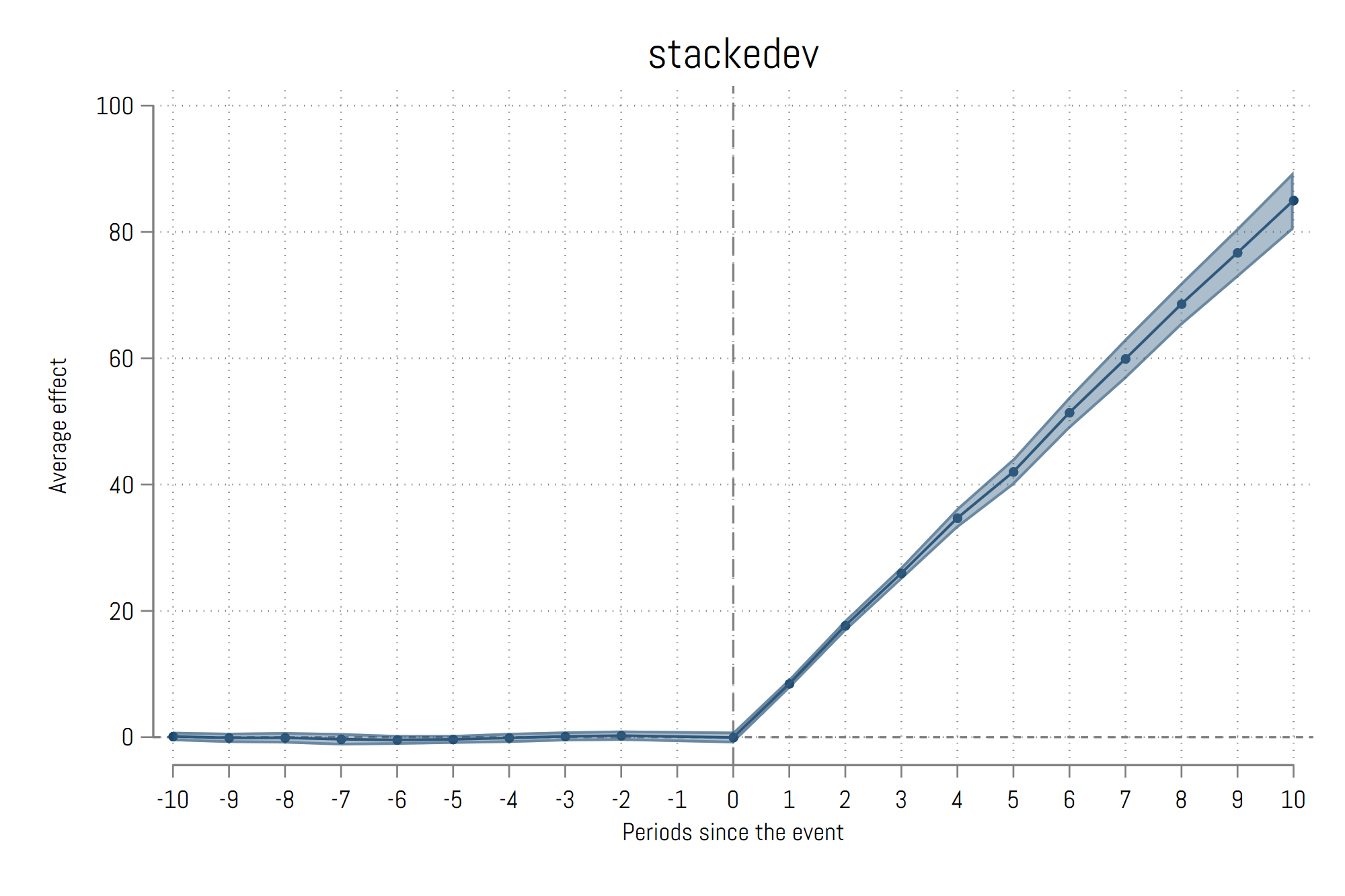
In order to plot the estimates we can use the event_plot
(ssc install event_plot, replace
) command where we restrict the figure to 10 leads and lags:
event_plot, default_look graph_opt(xtitle("Periods since the event") ytitle("Average effect") xlabel(-10(1)10) ///
title("stackedev")) stub_lag(L_#) stub_lead(F_#) trimlag(10) trimlead(10) together
And we get: