did2s (Gardner 2021)
Table of contents
Introduction
The did2s R package by Kyle Butts implements the method proposed by the Gardner 2021 paper Two-stage differences in differences. A detailed description is provided on the did2s website.
The key idea behind did2s is pretty simple and is clever implementation of the Frisch-Waugh-Lovell (FWL) theorem that should be familiar to many readers. In short, we can avoid the pathologies of staggered DiD settings by running two regressions (hence the name):
- Run a fixed-effects regression (including controls) on our outcome variable using only the untreated/not-yet-treated observations. Residualize the outcomes (i.e., subtract the predicted outcomes from the actual outcomes).
- Regress the residualized outcomes on the treatment dummies (or, time-to-treament dummies for an event study) using all obsevations to get the unbiased treatment effects.
A virtue of this two-step procedure is that it is very quick to estimate. Underneath the hood, did2s calls fixest, so all of the associated methods of the latter package are available (tabling, plotting, etc.). More importantly, it shares some syntax shortcuts/conventions that we should use for specifying our models. We’ll see some examples of this below.
Before continuing, it is worth noting that the did2s package also provides convenience functions for running and visualizing a range of DiD estimators (i.e., not just the method proposed by Gardner 2021). This makes it a very useful package to have in the applied econometrican’s R toolkit. We’ll save this functionality for the “All estimators” section, though. STILL NEED TO ADD THIS.
Installation and options
The package can be installed from CRAN.
install.packages("did2s") # Install (only need to run once or when updating)
library("did2s")          # Load the package into memory (required each new session)
The core estimating function is did2s() and it takes the following arguments:
did2s(data, yname, treatment, first_stage, second_stage, ...)
where
| Variable | Description |
|---|---|
| data | dataset |
| yname | outcome variable (character) |
| first_stage | 1st-stage regression forumula (controls & FEs) |
| second_stage | 2nd-stage regression formula (treatment indicator) |
| treatment | treatment dummy variable (character) |
| cluster_var | how to cluster SEs (character) |
| … | Additional arguments (bootstrapping, etc.) |
As mentioned above, did2s calls fixest underneath the hood and so
expects some the syntax conventions and shortcuts offered by the latter. The
most obvious cases are the use of the | fixed-effect slot in first_stage
formula, and the use of i() in the second_stage formula. We’ll illustrate
this directly with an example below. But you can take a look at the helpfile
(?did2s) for detailed information and additional examples.
Dataset
To demonstrate the package in action, we’ll use the fake dataset generated in the shared setup block here. Here’s a reminder of what the data look like.
head(dat)
#>   time id        y rel_time treat first_treat
#> 1    1  1 2.158289      -11 FALSE          12
#> 2    2  1 2.498052      -10 FALSE          12
#> 3    3  1 3.034077       -9 FALSE          12
#> 4    4  1 4.886266       -8 FALSE          12
#> 5    5  1 7.085950       -7 FALSE          12
#> 6    6  1 5.788352       -6 FALSE          12
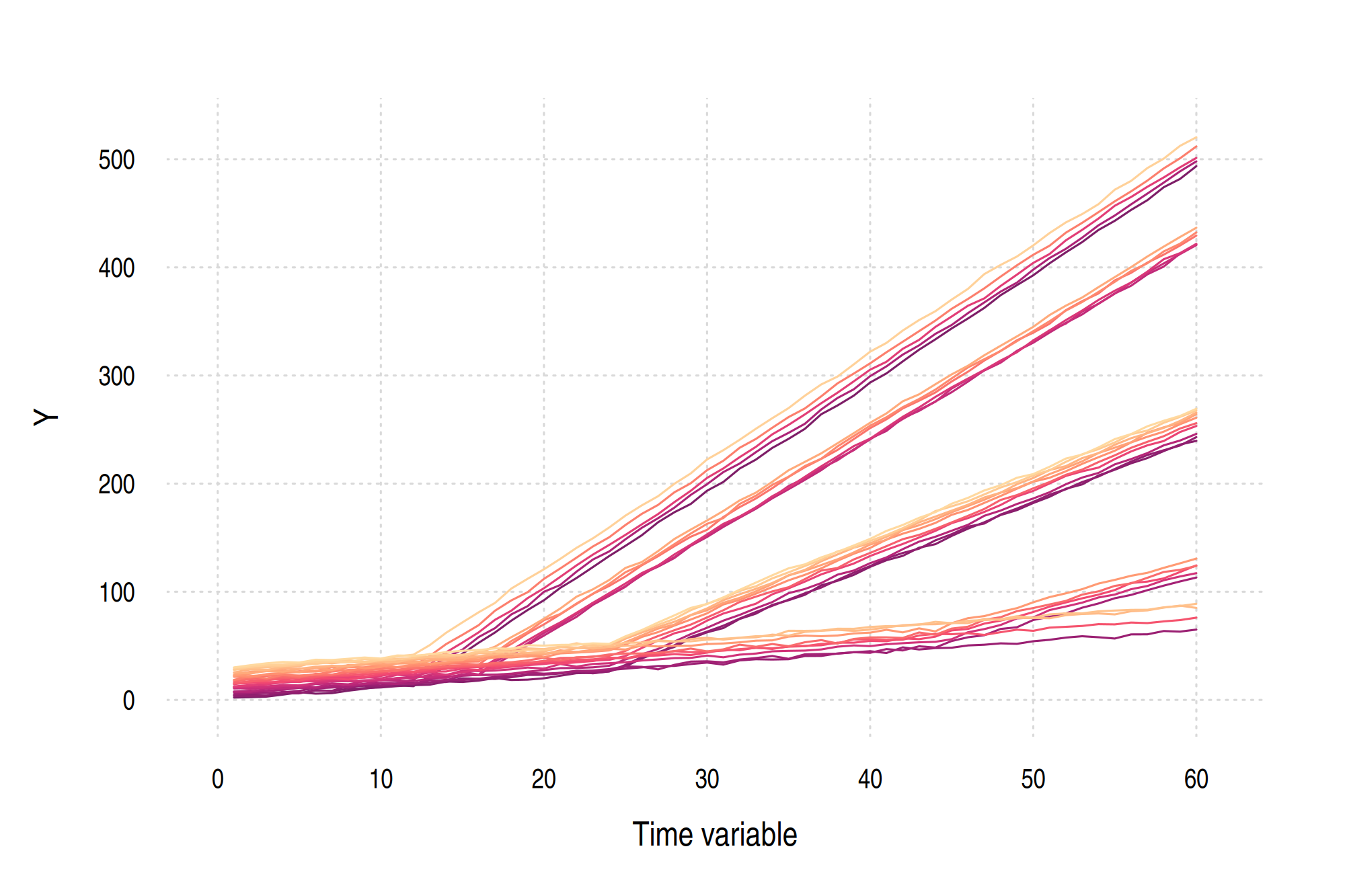
Or, in graph form.
Test the package
Remember to load the package (if you haven’t already).
library(did2s)
Let’s try the basic did2s() command on our fake dataset. We’ll start by
estimating a simple binary treatment effect, rather than a full event-study.
There are some things that I want to draw your attention to w.r.t. our first-
and second-stage regression arguments below. The first_stage formula uses |
to demarcate regular covariates (although theren’t any in this dataset) from the
fixed-effects slot. The second_stage formula invokes the i() operator to
create an indicator (factor) of our “treat” variable. Both of these syntax
features should be familiar to fixest users, but are worth underscoring all
the same.
did2s(
  data         = dat,
  yname        = "y",
  first_stage  = ~ 0 | id + time, # 0 b/c we have no controls in this dataset
  second_stage = ~ i(treat),      # binary treatment dummy (not an event-study)
  treatment    = "treat",
  cluster_var  = "id",
  )

#' Running Two-stage Difference-in-Differences
#' • first stage formula `~ 0 | id + time`
#' • second stage formula `~ i(treat)`
#' • The indicator variable that denotes when treatment is on is `treat`
#' • Standard errors will be clustered by `id`
#' OLS estimation, Dep. Var.: y
#' Observations: 1,800
#' Standard-errors: Custom
#'                   Estimate   Std. Error  t value  Pr(>|t|)
#' treat::FALSE -5.010000e-15 1.070000e-15 -4.69674 2.844e-06 ***
#' treat::TRUE   1.399854e+02 1.216437e+01 11.50782 < 2.2e-16 ***
#' ---
#' Signif. codes:  0 '***' 0.001 '**' 0.01 '*' 0.05 '.' 0.1 ' ' 1
#' RMSE: 80.9   Adj. R2: 0.425782
Okay, now let’s try a more realistic use-case by estimating a full event-study.
The only change we need to make vis-à-vis the previous regression is in the
second_stage formula. This time, we’ll use a relative time variable (AKA
time-to-treatment) rather than a binary treatment indicator. Note that I’m
specifying two reference periods via i(rel_time, ref = c(-1, Inf)). The first
(-1) sets all effects relative to the period immediately before treatment. The
second (Inf) establishes the “never-treated” control group for this dataset;
this reference value may differ for your own data. I’ll also go ahead and save
the resulting model object, since I plan to graph the corresponding event-study
plot below.
es_mod = did2s(
  data         = dat,
  yname        = "y",
  first_stage  = ~ 0 | id + time,
  second_stage = ~ i(rel_time, ref = -c(1, Inf)), # Use relative time var. for event-study
  treatment    = "treat",
  cluster_var  = "id"
  )

#' Running Two-stage Difference-in-Differences
#' • first stage formula `~ 0 | id + time`
#' • second stage formula `~ i(rel_time, ref = -c(1, Inf))`
#' • The indicator variable that denotes when treatment is on is `treat`
#' • Standard errors will be clustered by `id`

es_mod
#' OLS estimation, Dep. Var.: y
#' Observations: 1,800
#' Standard-errors: Custom
#' rel_time::-43  -0.049719   0.272847   -0.182224 0.8554282
#' rel_time::-42  -0.150764   0.196905   -0.765670 0.4439783
#' rel_time::-41   0.411294   0.419485    0.980472 0.3269918
#' rel_time::-40  -0.060809   0.285788   -0.212777 0.8315264
#' rel_time::-39  -0.104809   0.445865   -0.235069 0.8141833
#' <TRUNCATED>
#' ---
#' Signif. codes:  0 '***' 0.001 '**' 0.01 '*' 0.05 '.' 0.1 ' ' 1
#' RMSE: 25.7   Adj. R2: 0.939163
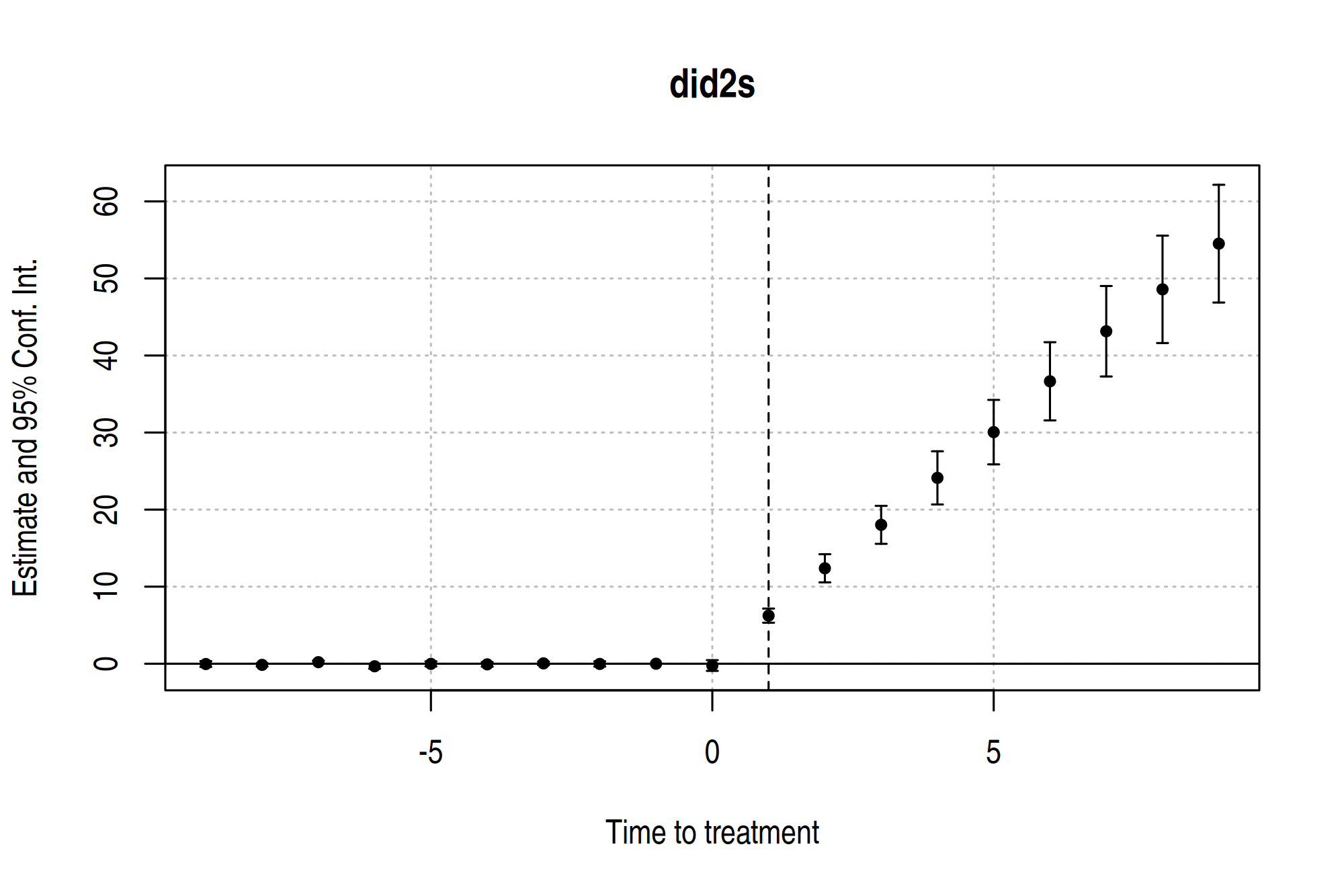
As I keep emphasizing, did2s is using fixest underneath the hood and all
of the latter methods apply. So we plot our event-study model using
fixest::iplot().
# fixest::iplot(es_mod)
# Vanilla option (above) is fine, but we can tweak a bit...
es_mod |>
  fixest::iplot(
    main     = "did2s",
    xlab     = "Time to treatment",
    drop     = "[[:digit:]]{2}",    # Drop any leads/lags greater than |9|
    ref.line = 1
  )
P.S. For those of you that would prefer a ggplot2 version of the above (base R) plot, check out ggfixest.