Bacon decomposition
Table of contents
- What is Bacon decomposition?
- The logic of the weights
- Manual recovery of weights
- So where do TWFE regressions go wrong?
This section has been updated and considerably improved thanks to Daniel Sebastian Tello Trillo.
Last updated: 16 May 2024
What is Bacon decomposition?
As discussed in the last example of the TWFE section, if we have different treatment timings with different treatment effects, it is not so obvious what pre and post are. Let us state this example again:
clear
local units = 3
local start = 1
local end   = 10

local time = `end' - `start' + 1
local obsv = `units' * `time'
set obs `obsv'

egen id	   = seq(), b(`time')
egen t 	   = seq(), f(`start') t(`end')

sort  id t
xtset id t

lab var id "Panel variable"
lab var t  "Time  variable"

gen D = 0
replace D = 1 if id==2 & t>=5
replace D = 1 if id==3 & t>=8
lab var D "Treated"

gen Y = 0
replace Y = D * 2 if id==2 & t>=5
replace Y = D * 4 if id==3 & t>=8

lab var Y "Outcome variable"
If we plot this:
twoway ///
	(connected Y t if id==1) ///
	(connected Y t if id==2) ///
	(connected Y t if id==3) ///
		,	///
		xline(4.5 7.5) ///
		xlabel(1(1)10) ///
		legend(order(1 "id=1" 2 "id=2" 3 "id=3"))
we get:
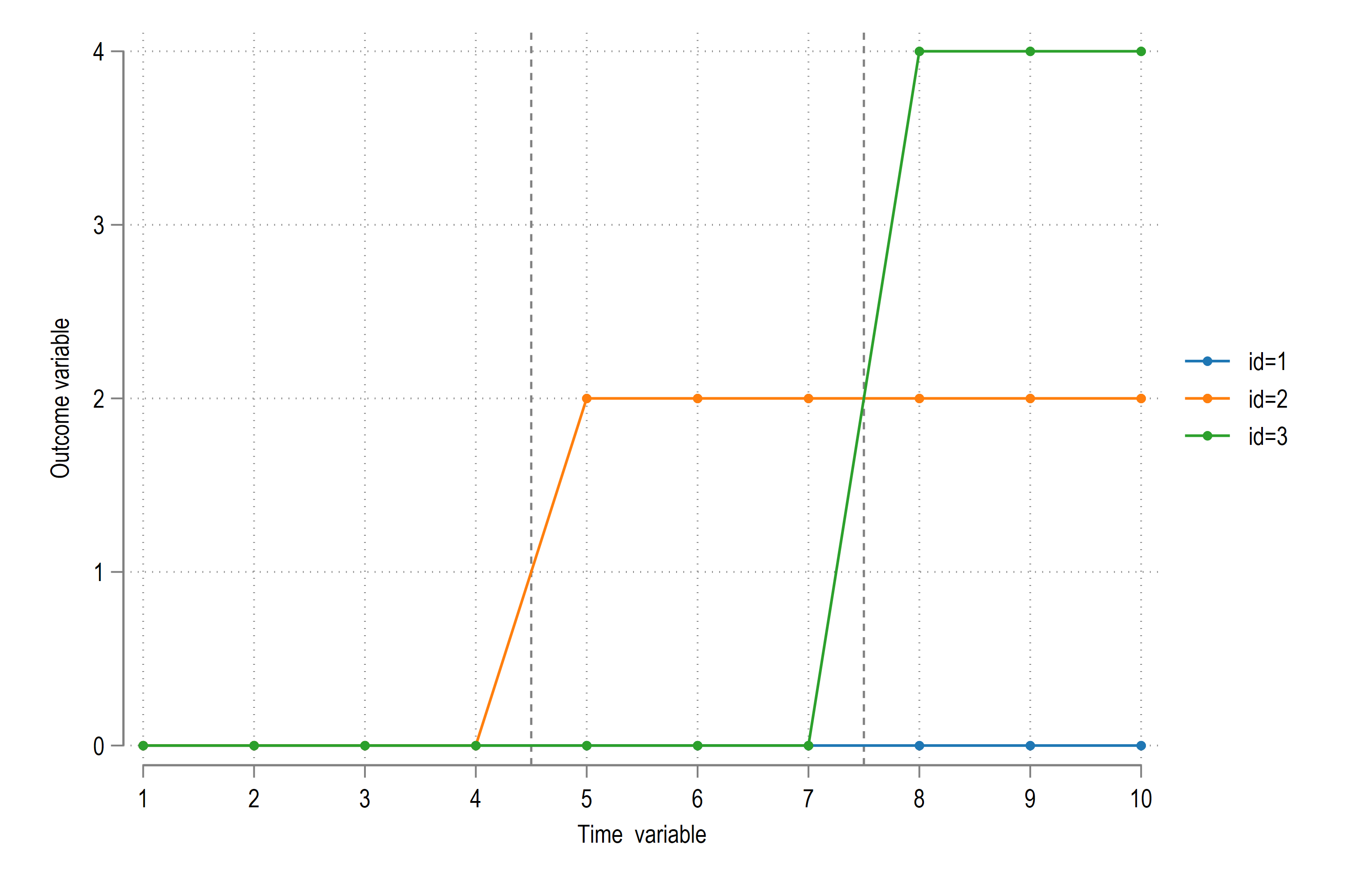
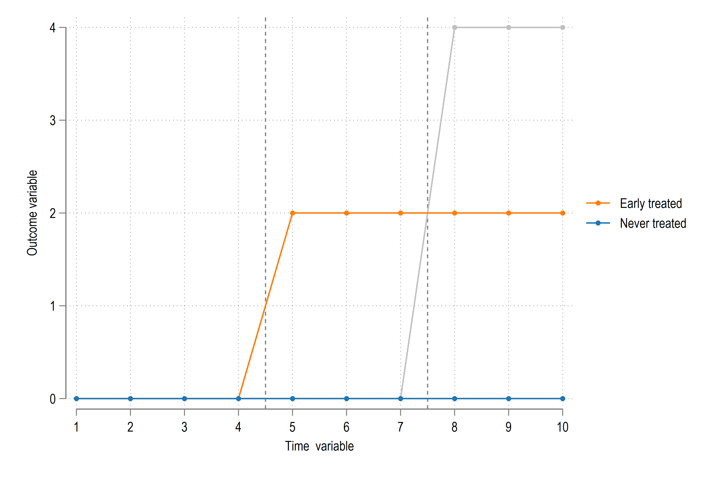
In the figure we can see that treatments occurs at two different points. The treatment to id=2 happens at \(t\)=5, while the treatment to id=3 happens at \(t\)=8. When the second treatment takes place, id=2 is already treated and is basically constant. So for id=3, id=2 is also part of the pre-treatment group especially if we just consider the time range \(5 \leq t \leq 10\). It is also not clear what the ATT in this case should be from just looking at the figure since we can no longer average out the treatment sizes as was the case with simpler examples discussed in section TWFE section. In order to recover this, we can run a simple specification:
xtreg Y D i.t, fe
reghdfe Y D, absorb(id t)   // alternative specification
which gives us an ATT of \(\hat{\beta}\) = 2.91. In summary this is the average treatment size after accounting for time and panel fixed effects.
Going back to the figure, this type of relative grouping of treated and not treated, and early and late treated, is part of the new DiD papers, just because each of these combinations plays its own role on the overall average \(\hat{\beta}\). This is exactly what Bacon decomposition tell us. It unpacks the \(\hat{\beta}\) coefficient as a weighted average \(\hat{\beta}\)s coefficients estimated from three distinct 2x2 groups:
- treated (\(T\)) versus never treated (\(U\))
- early treated (\(T^e\)) versus late control (\(C^l\))
- late treated (\(T^l\)) versus early control (\(C^e\))
In other words, the panel ids are split into different timing cohorts based on when the first treatment takes place and where it lies in relation to the treatment of other panel ids. The more the panel ids and differential treatment timings, the more the combinations of the above groups.
In our simple example, we have two treated panel ids: id=2 (early treated \(T^e\)) and id=3 (late treated \(T^l\)). The treated versus never treated can be further divided into early treated vs never treated (\(T^e\) vs \(U\)) and late treated vs never treated (\(T^l\) vs \(U\)). In total, four sets of values are estimated if there are three groups. Goodman-Bacon also uses a similar example in the paper.
Each set of values is essentially a basic 2x2 TWFE model, from which we recover two thing:
- A 2x2 (\(\hat{\beta}\)) parameter using classic TWFE.
- The weight of this parameter on the overall (\(\hat{\beta}^{DD}\)) as determined by its relative size in the data
We go back to these later. But first, let’s see what the bacondecomp command gives us:
bacondecomp Y D, ddetail
In the absence of controls, this is the only option we can use for running bacondecomp. At the end of the command, we get this figure:
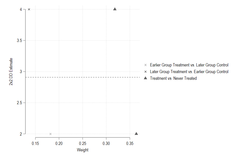
The figure shows four points for the three groups in our example. The treated versus never treated (\(T\) vs \(U\)) is shown as a triangle. Crosses represent late versus early treated (\(T^l\) vs \(T^e\)) combinations. The hollow circle represents the timing groups or early versus late treatment groups (\(T^e\) vs \(T^l\)).
The figure information is displayed in a table output:
Computing decomposition across 3 timing groups
including a never-treated group
------------------------------------------------------------------------------
           Y | Coefficient  Std. err.      z    P>|z|     [95% conf. interval]
-------------+----------------------------------------------------------------
           D |   2.909091   .3179908     9.15   0.000      2.28584    3.532341
------------------------------------------------------------------------------

Bacon Decomposition

+---------------------------------------------------+
|                      |         Beta   TotalWeight |
|----------------------+----------------------------|
|         Early_v_Late |            2   .1818181841 |
|         Late_v_Early |            4   .1363636317 |
|       Never_v_timing |  2.933333323   .6818181841 |
+---------------------------------------------------+
Here we get our weights and the 2x2 \(\beta\) for each group. The table tells us that (\(T\) vs \(U\)), which is the sum of the late and early treated versus never treated, has the largest weight, followed by early vs late treated, and lastly, late vs early treated.
Let’s look at the information that is stored:
ereturn list
The key matrix of interest is e(summdd):
mat list e(sumdd)
which gives us the following:
e(sumdd)[3,2]
                     Beta  TotalWeight
Early_v_Late            2    .18181818
Late_v_Early            4    .13636363
Never_v_ti~g    2.9333333    .68181818
From this matrix we can recover the \(\beta\):
display e(sumdd)[1,1]*e(sumdd)[1,2] + e(sumdd)[2,1]*e(sumdd)[2,2] + e(sumdd)[3,1]*e(sumdd)[3,2]
which gives us the original value of \(\beta\) = 2.909, as a weighted sum of the different 2x2 combinations of early, late, and never treated groups. This breakdown is essentially the core point of the Bacon Decomposition.
The logic of the weights
In this section, we will learn to recover the weights manually for our example. In order to do this we need to go through the equations defined in this paper:
Goodman-Bacon, A. (2021). Difference-in-differences with variation in treatment timing. Journal of Econometrics.
If you cannot access it, there are working paper versions floating around the internet (e.g. one here on NBER) plus there are also videos available on YouTube, for example, one here.
Let us start with Equation 3 in the paper which states that:
\[\hat{\beta}^{DD} = \frac{\hat{C}(y_{it},\tilde{D}_{it})}{\hat{V}^D} = \frac{ \frac{1}{NT} \sum_i{\sum_t{y_{it}\tilde{D}_{it}}}}{ \frac{1}{NT} \sum_i{\sum_t{\tilde{D}^2_{it}}}}\]This is basically a standard panel regression with fixed effects (see Greene or Wooldridge textbooks on panel estimations). Under the hood, a lot is going on in terms of symbols which we need to define. Let’s start with the basic ones:
- \(N\) = total panels because \(i = 1\dots N\)
- \(T\) = total time periods because \(t = 1\dots T\)
The symbol \(\tilde{D}_{it}\) is the demeaned value of \(D_{it}\) which is a dummy variable that equals one for the treated observations and zero otherwise. The ~ symbol is telling us to demean by time and panel means. In other words:
\[\tilde{D}_{it} = (D_{it} - D_i) - (D_{t} - \bar{\bar{D}})\]where
\[\bar{\bar{D}} = \frac{\sum_i{\sum_t{D_{it}}}}{NT}\]which is just the mean of all the observations. This specification is used to demean variables (to incorporate fixed effects). If we do demean or center the data, we can also recover the panel estimates using the standard reg command in Stata. In terms of syntax, this implies that, xtreg y i.t, fe is equivalent to reg tildey [check] (see Greene or Wooldridge).
So if we go to the \(\hat{\beta}^{DD}\) equation, \(\hat{V}^D\) is essentially the variance of \(D_{it}\). For our basic example, we can calculate the means manually (in double precision!):
egen double d_barbar=mean(D)

bysort id: egen double d_meani=mean(D)

bysort t: egen double d_meant=mean(D)

gen double d_tilde=(d-d_meani)-(d_meant-d_barbar)

gen double d_tilde_sq=d_tilde^2
| \(i\) | \(t\) | \(y\) | \(D\) | \(\bar{D}_i\) | \(\bar{D}_t\) | \(\bar{\bar{D}}\) | \(\tilde{D}_{it}\) | \(\tilde{D}^2_{it}\) |
|---|---|---|---|---|---|---|---|---|
| 1 | 1 | 0 | 0 | 0 | 0 | 0.3 | 0.3 | 0.09 |
| 1 | 2 | 0 | 0 | 0 | 0 | 0.3 | 0.3 | 0.09 |
| 1 | 3 | 0 | 0 | 0 | 0 | 0.3 | 0.3 | 0.09 |
| 1 | 4 | 0 | 0 | 0 | 0 | 0.3 | 0.3 | 0.09 |
| 1 | 5 | 0 | 0 | 0 | 0.33 | 0.3 | -0.03 | 0.0009 |
| 1 | 6 | 0 | 0 | 0 | 0.33 | 0.3 | -0.03 | 0.0009 |
| 1 | 7 | 0 | 0 | 0 | 0.33 | 0.3 | -0.03 | 0.0009 |
| 1 | 8 | 0 | 0 | 0 | 0.67 | 0.3 | -0.37 | 0.1369 |
| 1 | 9 | 0 | 0 | 0 | 0.67 | 0.3 | -0.37 | 0.1369 |
| 1 | 10 | 0 | 0 | 0 | 0.67 | 0.3 | -0.37 | 0.1369 |
| 2 | 1 | 0 | 0 | 0.6 | 0 | 0.3 | -0.3 | 0.09 |
| 2 | 2 | 0 | 0 | 0.6 | 0 | 0.3 | -0.3 | 0.09 |
| 2 | 3 | 0 | 0 | 0.6 | 0 | 0.3 | -0.3 | 0.09 |
| 2 | 4 | 0 | 0 | 0.6 | 0 | 0.3 | -0.3 | 0.09 |
| 2 | 5 | 2 | 1 | 0.6 | 0.33 | 0.3 | 0.37 | 0.1369 |
| 2 | 6 | 2 | 1 | 0.6 | 0.33 | 0.3 | 0.37 | 0.1369 |
| 2 | 7 | 2 | 1 | 0.6 | 0.33 | 0.3 | 0.37 | 0.1369 |
| 2 | 8 | 2 | 1 | 0.6 | 0.67 | 0.3 | 0.03 | 0.0009 |
| 2 | 9 | 2 | 1 | 0.6 | 0.67 | 0.3 | 0.03 | 0.0009 |
| 2 | 10 | 2 | 1 | 0.6 | 0.67 | 0.3 | 0.03 | 0.0009 |
| 3 | 1 | 0 | 0 | 0.3 | 0 | 0.3 | 0 | 0 |
| 3 | 2 | 0 | 0 | 0.3 | 0 | 0.3 | 0 | 0 |
| 3 | 3 | 0 | 0 | 0.3 | 0 | 0.3 | 0 | 0 |
| 3 | 4 | 0 | 0 | 0.3 | 0 | 0.3 | 0 | 0 |
| 3 | 5 | 0 | 0 | 0.3 | 0.33 | 0.3 | -0.33 | 0.1089 |
| 3 | 6 | 0 | 0 | 0.3 | 0.33 | 0.3 | -0.33 | 0.1089 |
| 3 | 7 | 0 | 0 | 0.3 | 0.33 | 0.3 | -0.33 | 0.1089 |
| 3 | 8 | 4 | 1 | 0.3 | 0.67 | 0.3 | 0.33 | 0.1089 |
| 3 | 9 | 4 | 1 | 0.3 | 0.67 | 0.3 | 0.33 | 0.1089 |
| 3 | 10 | 4 | 1 | 0.3 | 0.67 | 0.3 | 0.33 | 0.1089 |
where \(D\) = 1 if treated, \(\bar{D}_i\) is the average of \(D\) for each panel id \(i\), \(\bar{D}_t\) is the average of \(D\) for each \(t\), and \(\bar{\bar{D}}\) is the mean of the \(D\) column. \(\tilde{D}_{it}\) is calculated using the formula stated above and \(\tilde{D}^2_{it}\) is just its square term. Here the sum of the \(\tilde{D}^2_{it}\) column equals 2.20 which divided by \(NT\), or 3 x 10, equals 0.0733, which is the variance \(\hat{V}^D\).
We can also recover \(\hat{V}^D\) as follows in Stata:
 xtreg D i.t , fe

 cap drop Dtilde
 predict double Dtilde, e

 sum Dtilde
 scalar VD = (( r(N) - 1) / r(N) ) * r(Var)
or manually using the standard variance/covariance method:
gen double numerator_1=y*d_tilde
egen double numerator=mean(numerator_1)
egen double denominator=mean(d_tilde_square)

sum denominator
where we can view the value by typing display VD. Here we should get 0.0733 as expected.
In the paper, three additional formulas are provided for dealing with the three groups in our example. These are defined as follows in Equation 10:
- Early treatment versus late control (\(T^e\) vs \(C^l\))
- Late treatment versus early control (\(T^l\) vs \(C^e\))
- Treated versus untreated (\(T\) vs \(U\)):
where \(j = \{e,l\}\) or early and late treatment groups.
The \(s\) are basically the weights that the command bacondecomp recovers, that are also displayed in the table. And since there is also a 2x2 \(\hat{\beta}\) coefficient associated with each 2x2 group, the weights have two properties:
- They add up to one or:
- The overall \(\hat{\beta}^{DD}\) is a weighted sum of the 2x2 \(\hat{\beta}\) parameters:
Next step, we need to define all the new symbols. But before we do that, we need to get the logic straight. And for this, we start with the original visual:
Here we can see that the never treat group, \(U\), which is id=1, runs for 10 periods and gets treatment in zero periods. The early treated group (id=2), \(T^e\), runs for six periods starting at 5 and ending at 10, while the late treated group (id=3), \(T^l\) runs for 3 periods from 8 till 10. These numbers tell us how many time periods a group stays treated. The share of these values out of the total observations \(T\) gives us \(D^e = 6/10\) and \(De = 3/10\) values. This tells us how much weight each panel group exerts in the total observations. A group that stays treated for longer will (and should) have a larger influence on the ATT.
The next set of values are \(n_e\), \(n_l\), and \(n_U\), which are the sample size of the groups in the total time periods. Since our panel is fully balanced, and there are three groups, these values equal \(n_e = n_l = n_U = 1/3\) (check this). Each 2x2 contains a pair of the \(\{e,l,U\}\) group, the sum of \(n\) shares essentially weigh the relative size of the two panel ids in the group sample in the total observations.
The last unknown value is of the form \(n_{ab}\) which is the share of the time of treatment units in a group time, or
\[n_{ab} = \frac{n_a}{n_a + n_b}\]The aim of this value is to weight the relative share of treatment within each group. If a treatment takes place in a very small fraction of the time, or a very large fraction of the time, then its weight in the overall \(\hat{\beta}\) will be reduced. In other words, more evenly spaced treatments in each group are given a higher preference.
From the share formulas above, we can see that it is all about accouting for all sorts of weights that are then applied to the recovered 2x2 \(\hat{beta}\) of each group.
Manual recovery of weights
Let’s start with the manual recovery process.
Late treatment vs early control
In order to visualize late treated versus early control, we generate the following control and draw the graph:
cap drop tle
gen tle = .
replace tle = 0 if t>=5
replace tle = 1 if t>=8 & id==3

twoway ///
	(line Y t if id==1, lc(gs12)) ///
	(line Y t if id==2, lc(gs12)) ///
	(line Y t if id==3, lc(gs12)) ///
	(line Y t if id==3 & tle!=.) ///
	(line Y t if id==2 & tle!=.) ///
		,	///
		xline(4.5 7.5) ///
		xlabel(1(1)10) ///
		legend(order(4 "Late treated" 5 "Early control"))
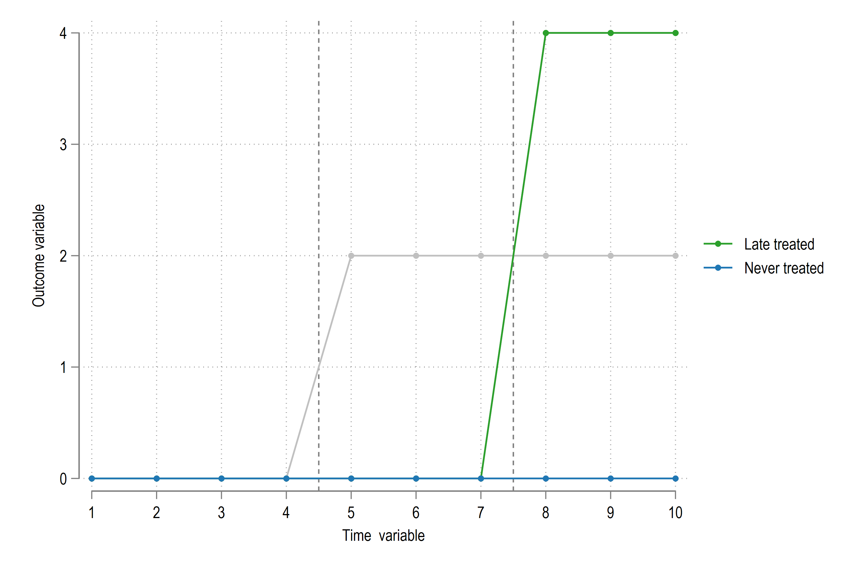
and we get this figure:
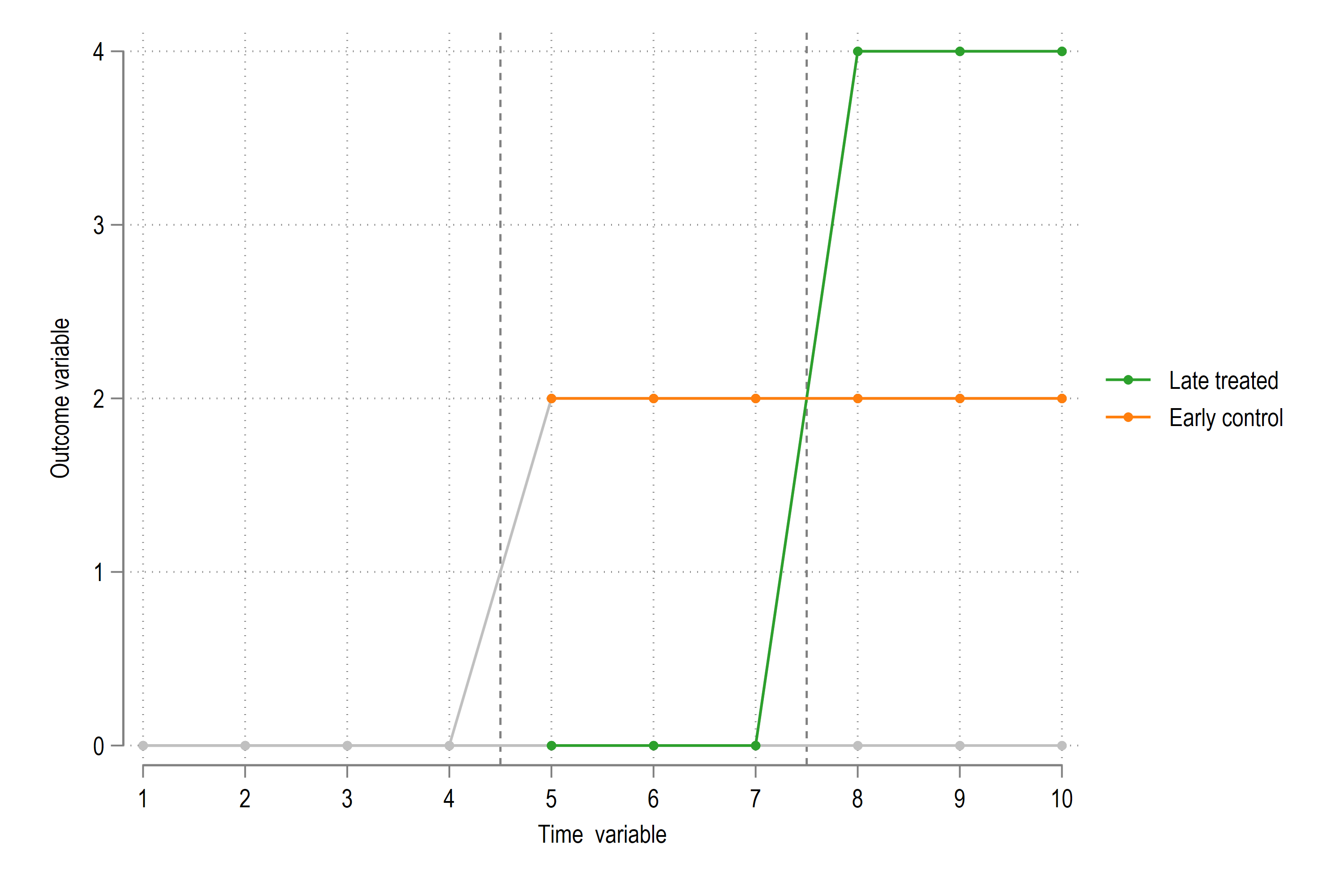
So what is happening in this figure? We see that the id=2 variable which was treated earlier is flat, while the id=3 variable gets a treatment. Here we are saying that rather than calculate the TWFE estimator over the whole sample, we generate it for just id=3 and use id=2 as the control since it is stable in the \(t\) = 5 to 10 interval.
Since we know from above, that the formula for this setting is:
\[s_{le} = \frac{ ((n_e + n_l)\bar{D}_e))^2 n_{el} (1 - n_{el}) \frac{\bar{D}_l}{\bar{D}_e} \frac{\bar{D}_e - \bar{D}_l}{\bar{D}_e} }{\hat{V}^D}\]we can define the values manually as follows:
scalar De  = 6/10  // share of early treated in all sample
scalar Dl  = 3/10  // share of late treated in all sample
scalar nl = 1/3    // relative group size of late
scalar ne = 1/3    // relative group size of early
scalar nel = 3/6   // share of treatment periods in group sample
where the last scalar nel is the share of treatment which is 3 periods in the total group time horizon of 6 time periods. Here we can recover the weights as follows:
display "weight_le = " (((ne + nl) * (De))^2 * nel * (1 - nel) * (Dl / De) * ((De - Dl)/(De)) ) / VD
which gives us a value of 0.136.
Since we already have the sample defined, we can also recover the 2x2 TWFE parameter:
xtreg Y D i.tle if (id==2 | id==3), fe robust
which gives us a value of \(D\) = 4. Since we don’t have time or panel fixed effects or gaussian errors, we can also see from the figure that the change in id=3 is 4 units, while id=2 stays constant so the change is 0.
Compare these values to the bacondecomp table shown above and you will that these values exactly match the table values.
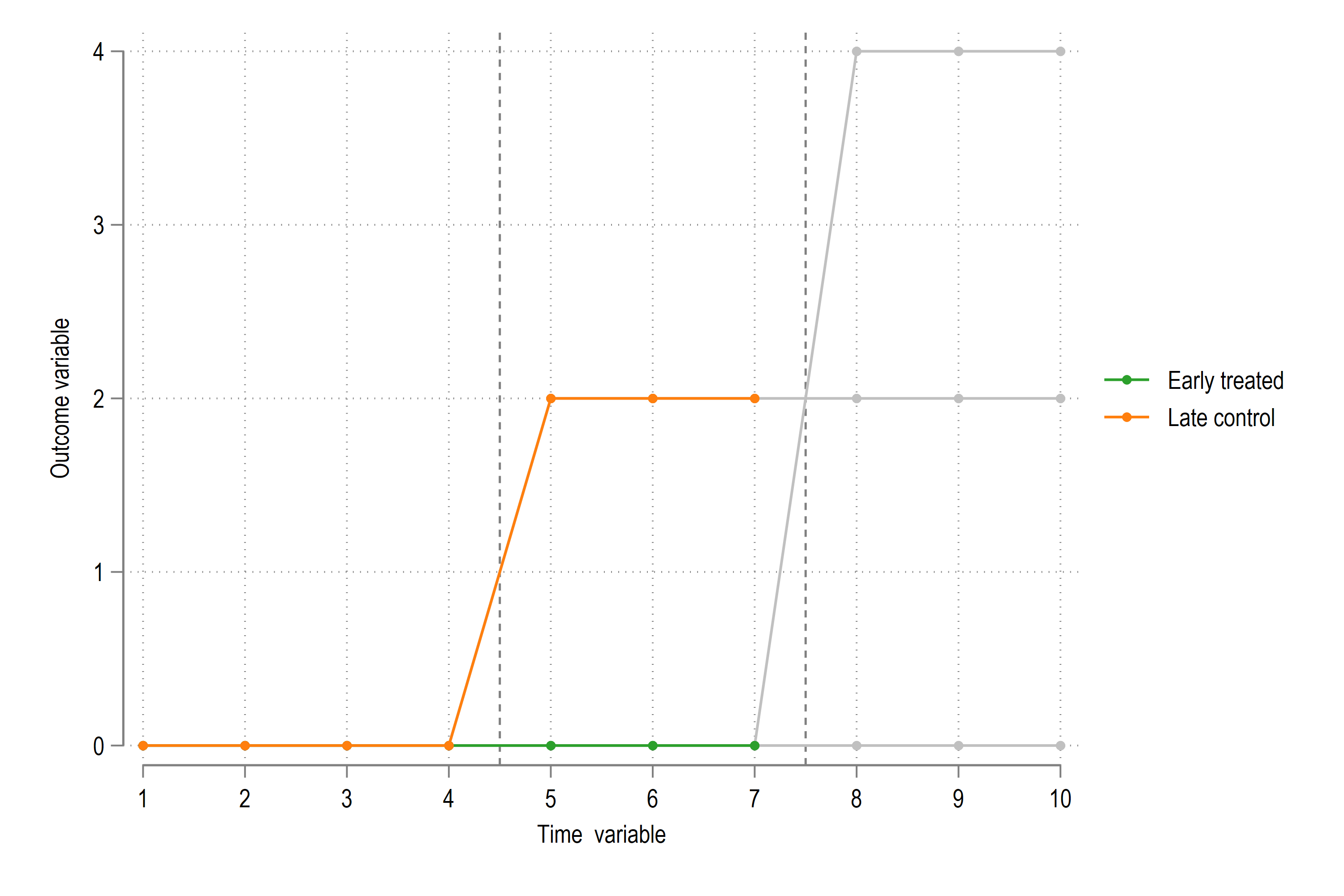
Early treatment vs late control
Now let’s flip this situation. Where we take the late treated variable as the control for the early treated group.
twoway ///
	(line Y t if id==1, lc(gs12)) ///
	(line Y t if id==2, lc(gs12)) ///
	(line Y t if id==3, lc(gs12)) ///
	(line Y t if id==3 & tel!=.) ///
	(line Y t if id==2 & tel!=.) ///
		,	///
		xline(4.5 7.5) ///
		xlabel(1(1)10) ///
		legend(order(4 "Early treated" 5 "Late control"))
From the figure, we can see that this falls in this range:
and we recover the weights for the share:
scalar De  = 6/10  // share of late treated in all sample
scalar Dl  = 3/10  // share of early treated in all sample

scalar nl = 1/3    // relative group size of late
scalar ne = 1/3    // relative group size of early
scalar nle = 3/6   // share of treatment periods in group sample. why is it 3/6 and not 3/7?

display "weight_el = " (((ne + nl) * (1 - Dl))^2 * (nle * (1 - nle)) * ((De - Dl)/(1 - Dl)) * ((1 - De)/(1 - Dl))) / VD

xtreg Y D i.tel if (id==2 | id==3), fe robust
which gives us a value of 0.182 and a \(\beta\)coefficient of 2. Again this values can be compared with the bacondecomp table above.
** Treated versus not treated **
Next we compare the two treated groups (early and late) with the not treated group:
cap drop ten
gen ten = .
replace ten = 0 if id==1
replace ten = 1 if id==2

twoway ///
	(line Y t if id==1, lc(gs12)) ///
	(line Y t if id==2, lc(gs12)) ///
	(line Y t if id==3, lc(gs12)) ///
	(line Y t if id==2 & ten!=.) ///
	(line Y t if id==1 & ten!=.) ///
		,	///
		xline(4.5 7.5) ///
		xlabel(1(1)10) ///
		legend(order(4 "Early treated" 5 "Never treated"))

cap drop tln
gen tln = .
replace tln = 0 if id==1
replace tln = 1 if id==3

twoway ///
	(line Y t if id==1, lc(gs12)) ///
	(line Y t if id==2, lc(gs12)) ///
	(line Y t if id==3, lc(gs12)) ///
	(line Y t if id==3 & tln!=.) ///
	(line Y t if id==1 & tln!=.) ///
		,	///
		xline(4.5 7.5) ///
		xlabel(1(1)10) ///
		legend(order(4 "Late treated" 5 "Never treated"))
We can recover the coefficients as follows:
xtreg Y D i.t if (id==1 | id==2), fe robust		// early
xtreg Y D i.t if (id==1 | id==3), fe robust		// late
which gives us 2 and 4 for early and late respectively. And we get the shares as follows:
scalar Dl  = 3/10  // share of late treated in all sample
scalar De  = 6/10  // share of early treated in all sample

scalar ne = 1/3    // relative group size of late
scalar nl = 1/3    // relative group size of late
scalar nU = 1/3    // relative group size of early

scalar nlU = 3/10   // share of treatment periods in group sample.
scalar neU = 6/10   // share of treatment periods in group sample.

display "weight_eU = " ((ne + nU)^2 * (neU * (1 - neU)) * (De * (1 - De))) / VD
display "weight_lU = " ((nl + nU)^2 * (nlU * (1 - nlU)) * (Dl * (1 - Dl))) / VD
where the shares equal 0.3636 and 0.31818 respectively. If we add these up, they come out to 0.68181. This number is not exactly the same number shown in the bacondecomp table, but here we can see that this group has the highest weight as expected.
We can also recover the respective betas as follows
// Early vs Never
xtreg Y D i.t if (id==1 | id==2), fe robust

// Late vs Never
xtreg Y D i.t if (id==1 | id==3), fe robust
We can also check manually the weighted average of the beta coefficients and compare it with the regression coefficient:
// manual
display 4*.31818182 + 2*.36363636 + 2*.18181818 + 4*.13636364

// regression
reghdfe Y D, absorb(id t)
and we get the same estimate of 2.909.
So where do TWFE regressions go wrong?
Up till now, we have looked at examples, where we have a discrete jump in the treatment. In our very simple example, we ran some regressions to estimate treatment effects on afew observations that we could also recovery manually. We also went through the Bacon decomposition which told us how the \(\hat{\beta}\) coefficient is a weighted sum of various 2x2 treated and untreated groups.
But where does the TWFE model go wrong? Here we need to change the treatment effects a bit. Rather than discrete jumps, we allow treatments to take place across cohorts of units at some point in time and we let th treatment effects gradually increase over time.
Rather than using our simple example, let’s scale up the problem set a bit by adding multiple panel ids.
clear
local units = 30
local start = 1
local end   = 60

local time = `end' - `start' + 1
local obsv = `units' * `time'
set obs `obsv'

egen id	   = seq(), b(`time')
egen t 	   = seq(), f(`start') t(`end')

sort  id t
xtset id t

lab var id "Panel variable"
lab var t  "Time  variable"
Here we have 30 units (\(i\)) and 60 time periods (\(t\)). You can increase these to which ever magnitude. We will also do this later for testing.
We can also fix the seed in case you want replicate exactly what we have here:
set seed 13082021
You can of course don’t need to do this but it helps some people following the code and the scripts. We will remove this later for testing as well.
Let’s now generate some dummy variables:
cap drop Y
cap drop D
cap drop cohort
cap drop effect
cap drop timing

gen Y 	   = 0		// outcome variable
gen D 	   = 0		// intervention variable
gen cohort = .  	// total treatment variables
gen effect = .		// treatment effect size
gen timing = .		// when the treatment happens for each cohort
First we need to define the cohorts. These are groups of \(i\)s that get treatment at the same time. Think, for example, US states where some states are given treatment simultaneously, then another cohort and so on.
What we do here, is that we randomly assign a cohort. We can have as many cohorts (< \(i\)) as we want. But we add a cohort=0, that we will later use as the cohort that is never treated (we won’t do this now). Let’s say we want to generate five cohorts:
levelsof id, local(lvls)
foreach x of local lvls {
	local chrt = runiformint(0,5)
	replace cohort = `chrt' if id==`x'
}
Now we need to define two things for each cohort: (a), what is the treatment “effect” size, and (b), when the treatment happens, or the “timing” variable.
Let’s automate this:
levelsof cohort , local(lvls)  //  let all cohorts be treated for now
foreach x of local lvls {

	// (a) effect

	local eff = runiformint(2,10)
		replace effect = `eff' if cohort==`x'

	// (b) timing

	local timing = runiformint(`start' + 5,`end' - 5)
	replace timing = `timing' if cohort==`x'
		replace D = 1 if cohort==`x' & t>= `timing'
}
Here we generate a effect size for each cohort as a random integer between 2 and 10. Could be any number range which can also be on the continuous range.
The timing for each cohort is also randomly generated in the interval t=5 and t=55. This is just to make sure treatment cohorts are not very dominant, only exist for a couple of periods.
Last step, generate the outcome effects:
replace Y = id + t + cond(D==1, effect * (t - timing), 0)
Let’s graph it and see what the data looks like:
levelsof cohort
local items = `r(r)'

local lines
levelsof id

forval x = 1/`r(r)' {

	qui summ cohort if id==`x'
	local color = `r(mean)' + 1
	colorpalette tableau, nograph

	local lines `lines' (line Y t if id==`x', lc("`r(p`color')'") lw(vthin))	||
}

twoway ///
	`lines', legend(off)
which gives us:
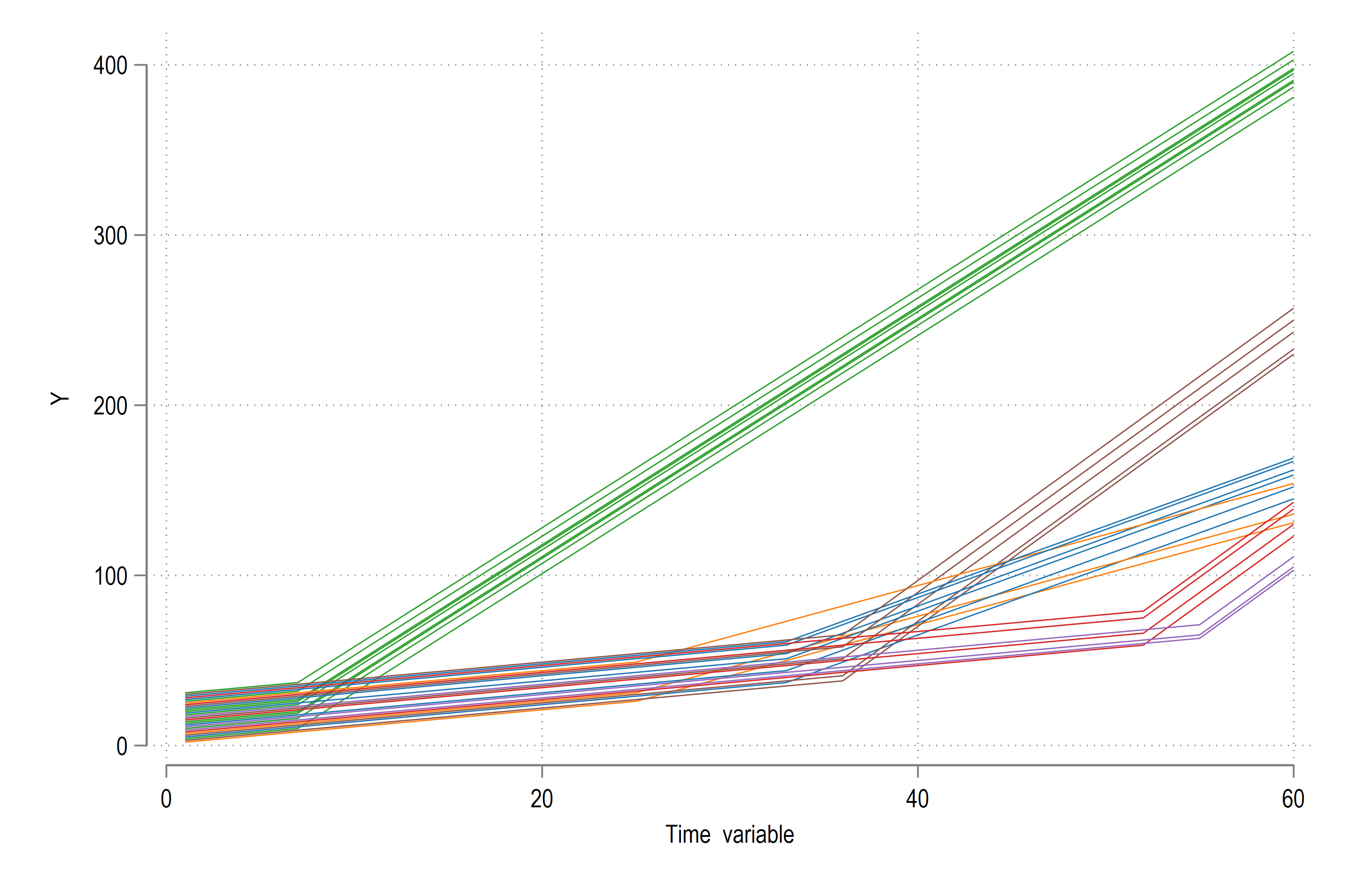
Each cohort is given a different color. This is passed on to the line graph via the colorpalette package.
In the figure we see that the green cohort gets treated early and contains a lot of ids. Orange is next but has few ids. Simiarly red and purple at the last ones to get treated. Regardless of being treated later or earlier, the effect of the treatment is positive. But what happens, when we run a TWFE regression?
xtreg Y i.t D, fe
Check the D coefficient. It is negative! We can also run it as follows using the reghdfe package:
reghdfe Y D, absorb(id t)
I have pasted the reghdfe regression output below (xtreg output was too large):
(MWFE estimator converged in 2 iterations)

HDFE Linear regression                            Number of obs   =      1,800
Absorbing 2 HDFE groups                           F(   1,   1710) =      59.04
                                                  Prob > F        =     0.0000
                                                  R-squared       =     0.8359
                                                  Adj R-squared   =     0.8273
                                                  Within R-sq.    =     0.0334
                                                  Root MSE        =    39.7334

------------------------------------------------------------------------------
           Y | Coefficient  Std. err.      t    P>|t|     [95% conf. interval]
-------------+----------------------------------------------------------------
           D |  -25.93176   3.374793    -7.68   0.000    -32.55092    -19.3126
       _cons |   114.9349   1.997427    57.54   0.000     111.0172    118.8525
------------------------------------------------------------------------------

Absorbed degrees of freedom:
-----------------------------------------------------+
 Absorbed FE | Categories  - Redundant  = Num. Coefs |
-------------+---------------------------------------|
          id |        30           0          30     |
           t |        60           1          59     |
-----------------------------------------------------+
This is obviously wrong since we know for sure that the treatments are positive. So what is going on? Let’s check using the Bacon decomposition:
bacondecomp Y D, ddetail
which gives us this graph:
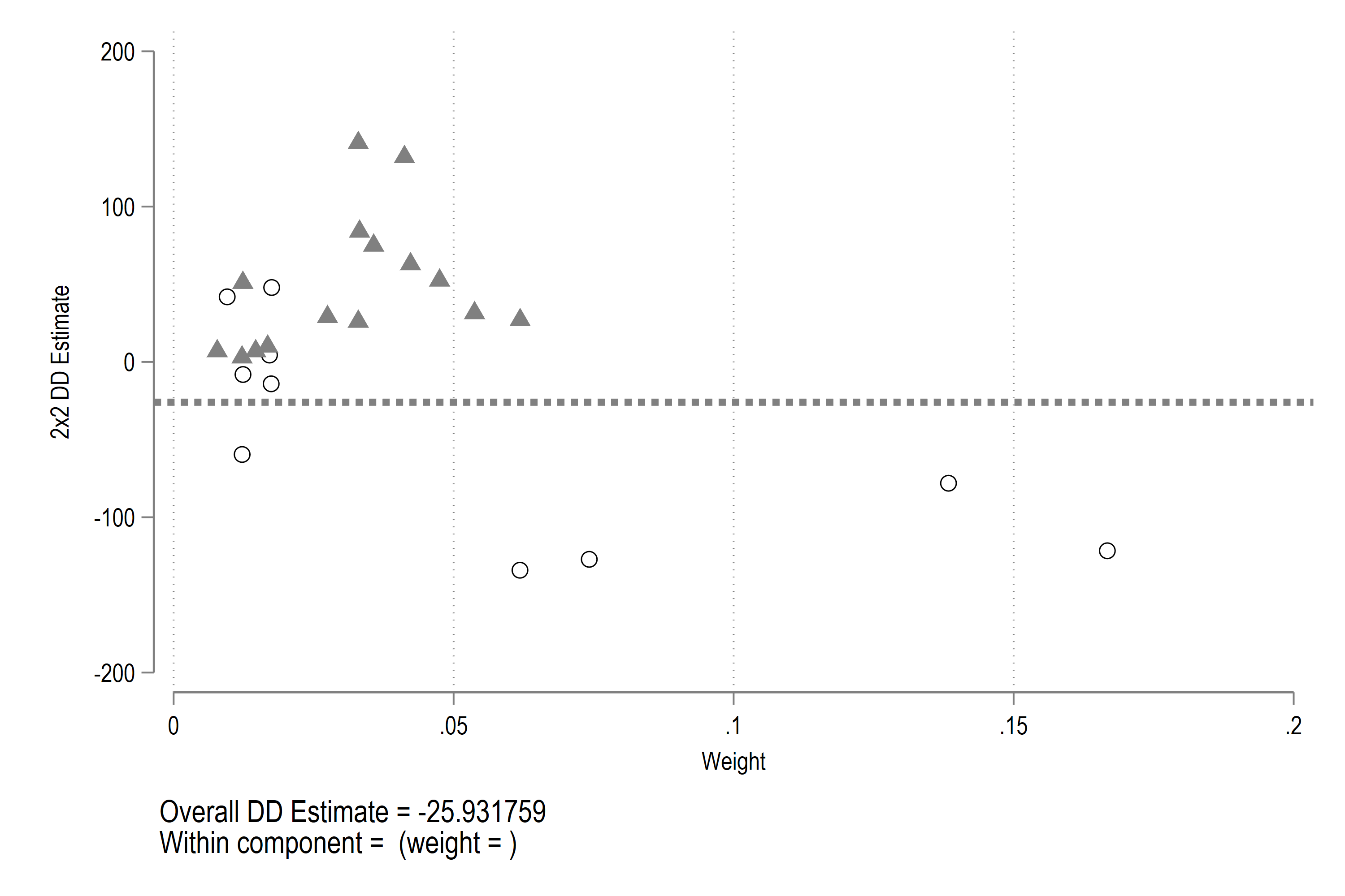
with details provided in the following output:
Computing decomposition across 6 timing groups
------------------------------------------------------------------------------
           Y | Coefficient  Std. err.      z    P>|z|     [95% conf. interval]
-------------+----------------------------------------------------------------
           D |  -25.93176   3.374793    -7.68   0.000    -32.54623   -19.31729
------------------------------------------------------------------------------

Bacon Decomposition

+---------------------------------------------------+
|                      |         Beta   TotalWeight |
|----------------------+----------------------------|
|         Early_v_Late |           51   .0123657302 |
|         Late_v_Early |         -127   .0741943846 |
|         Early_v_Late |           75   .0357232214 |
|         Late_v_Early |       -121.5   .1667083601 |
|         Early_v_Late |            7   .0146556807 |
|         Late_v_Early |          4.5   .0170982933 |
|         Early_v_Late |           84   .0332042752 |
|         Late_v_Early |          -78   .1383511554 |
|         Early_v_Late |           10   .0167929674 |
|         Late_v_Early |           48   .0174926737 |
|         Early_v_Late |            3   .0122130672 |
|         Late_v_Early |           42   .0095414589 |
|         Early_v_Late |          132   .0412191018 |
|         Late_v_Early |         -134   .0618286496 |
|         Early_v_Late |           26   .0329752828 |
|         Late_v_Early |           -8   .0123657302 |
|         Early_v_Late |           27   .0618795396 |
|         Late_v_Early |          -14   .0174036209 |
|         Early_v_Late |         52.5   .0474952625 |
|         Late_v_Early |        -59.5   .0122130672 |
|         Early_v_Late |  60.01138465   .1642784771 |
+---------------------------------------------------+
It is this decomposition and the negative weights that form the basis for the estimators in the new DiD packages that are discussed in sections below.