did (Callaway and Sant’Anna 2021)
Table of contents
Introduction
The did R package was developed by Brantly Callaway and Pedro Sant’Anna to accompany their 2021 paper Difference-in-Differences with multiple time periods (henceforth CS21).
CS21 provides an extremely flexible framework for estimating DiD-style regressions and can yield valid estimands in cases where other packages/routines struggle. At the heart of CS21—and thus the did package—is a fully saturated set of group (i.e., cohort) x time interactions. The idea is to estimate each of these interactions relative to a valid control group (by default, the never-treated units) and thus yield individual average treatment effects (ATTs). We can then aggregate these individual ATTs along different dimensions to yield “summary” results of interest. For example, we can aggregate dynamically (i.e., over time periods) to get the equivalent event-study coefficients.
If this level of generality and flexibility sounds like it requires a lot of work, that’s because it does. did does a great deal under the hood and I haven’t even talked about the way it computes the individual ATTs. (TL;DR it uses a “doubly-robust” approach by default, since CS21 proves the equivalence conditions for estimating by regression or inverse probability weighting.) But the package is very user-friendly and suprisingly nimble. A lot of work has gone into making estimation fast, with considerable speed gains unlocked through C++ optimization.
Installation and options
The package can be installed from CRAN.
install.packages("did") # Install (only need to run once or when updating)
library("did")          # Load the package into memory (required each new session)
The typical workflow for did involves two consecutive function calls.
agg_gt(): Estimate the individual (group x time) ATTs.aggte(): Aggregate the ATTs along the dimension of interest. For example, we can useaggte(..., type = "dynamic")to aggregate ATTs along the relative time dimension and thus obtain an event study.
Let’s quickly take a look at the main arguments for these two functions:
att_gt(yname, tname, idname, gname, xformla, data, ...)
where
| Variable | Description |
|---|---|
| yname | outcome variable (character) |
| tname | time variable (character) |
| idname | panel id variable (character) |
| gname | group or cohort variable defining a common first period (character) |
| xformla | addtional control variables (formula, optional) |
| data | dataset |
| … | Additional arguments (estimation method, DiD control group, etc.) |
and
aggte(model, type, ...)
where
| Variable | Description |
|---|---|
| model | model object resulting from the att_gt() call above |
| type | type of aggregation to compute, e.g. “group” or “dynamic” (character) |
| … | Additional arguments (clustering, bootsrapping, etc.) |
Again, did is extremely flexible and allows for a ton of additional
arguments beyond those presented here, including everything from treatment
anticipation to clustered or bootstrapped SEs. See the relevant helpfiles
(?att_gt and
?aggte)
for more information. Lastly, the did website contains a
series of extremely helpful user guides
(i.e., vignettes) that not only demonstrate how to use the package, but also
help users to think through the issues of DiD estimation more generally.
Dataset
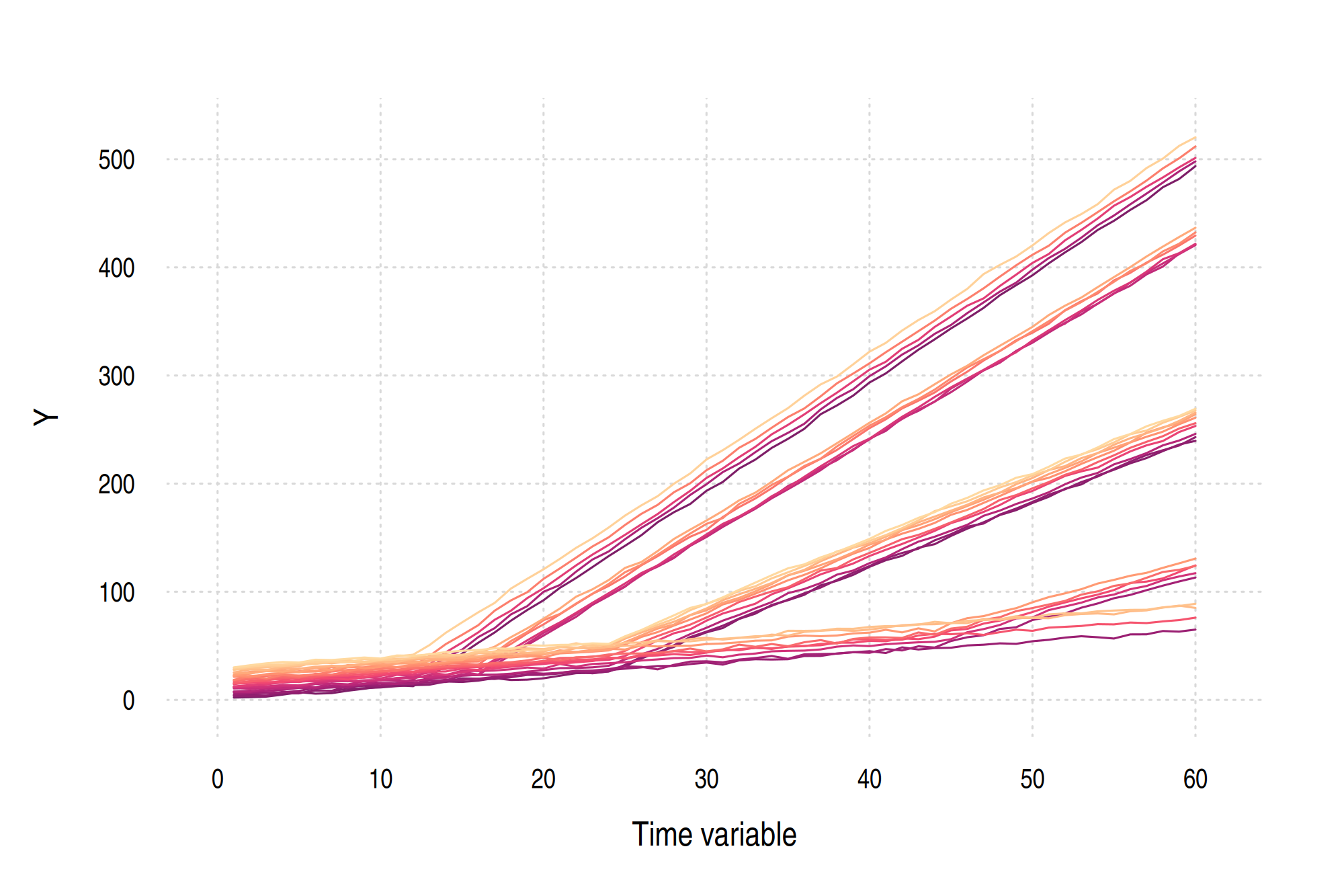
To demonstrate the package in action, we’ll use the fake dataset generated in the shared setup block here. Here’s a reminder of what the data look like.
head(dat)
#>   time id        y rel_time treat first_treat
#> 1    1  1 2.158289      -11 FALSE          12
#> 2    2  1 2.498052      -10 FALSE          12
#> 3    3  1 3.034077       -9 FALSE          12
#> 4    4  1 4.886266       -8 FALSE          12
#> 5    5  1 7.085950       -7 FALSE          12
#> 6    6  1 5.788352       -6 FALSE          12
Or, in graph form.
Test the package
Remember to load the package (if you haven’t already).
library(did)
Okay, let’s run the first of our two complementary functions, att_gt(), to get
the (group x time) ATTs. The below function call should be pretty
self-explanatory and only takes a second or two to run. But I do want to
highlight the fact that we specify control_group = "notyettreated" (rather
than the “nevertreated” default). This is just an artefact of our simulated
dataset, which doesn’t provide enough never-treated units for the underlying
CS21 estimation procedure. If you omitted this argument (as I did originally),
then the functional will return a helpful prompt to fix the problem.
cs21 = att_gt(
    yname         = "y",
    tname         = "time",
    idname        = "id",
    gname         = "first_treat",
  # xformla       = NULL,            # No additional controls in this dataset
    control_group = "notyettreated", # Too few groups for "nevertreated" default
    clustervars   = "id",
    data          = dat
    )
cs21

#' Call:
#' att_gt(yname = "y", tname = "time", idname = "id", gname = "first_treat",
#'     data = dat, control_group = "notyettreated", clustervars = "id")
#'
#' Reference: Callaway, Brantly and Pedro H.C. Sant'Anna.  "Difference-in-
#' Differences with Multiple Time Periods." Journal of Econometrics, Vol. 225,
#' No. 2, pp. 200-230, 2021. <https://doi.org/10.1016/j.jeconom.2020.12.001>,
#' <https://arxiv.org/abs/1803.09015>
#'
#' Group-Time Average Treatment Effects:
#'  Group Time ATT(g,t) Std. Error [95% Simult.  Conf. Band]
#'     12    2   0.3932     0.6474       -1.4985      2.2849
#'     12    3  -0.9038     0.7147       -2.9919      1.1844
#'     12    4   0.6265     0.5265       -0.9118      2.1648
#'     12    5   0.7449     0.5280       -0.7979      2.2876
#'     12    6  -1.4944     0.5348       -3.0571      0.0683
#' <TRUNCATED>
With our ATTs in hand, we can now proceed to our second function, aggte(),
to compute the aggregate quantities of interest. In this case, I’ll specify
“dynamic” aggregation to get an event-study (i.e., ATTs aggregated across
relative time-to-treatment periods). I’ll also limit the study extent around
the treatment date to 10 leads and 10 lags.
cs21_es = aggte(cs21, type = "dynamic", min_e = -10, max_e = 10)
cs21_es
#' Call:
#' aggte(MP = cs21, type = "dynamic", min_e = -10, max_e = 10)
#'
#' Reference: Callaway, Brantly and Pedro H.C. Sant'Anna.  "Difference-in-Differences with Multiple Time Periods." Journal of Econometrics, Vol. 225, No. 2, pp. 200-230, 2021. <https://doi.org/10.1016/j.jeconom.2020.12.001>, <https://arxiv.org/abs/1803.09015>
#'
#'
#' Overall summary of ATT's based on event-study/dynamic aggregation:
#'     ATT    Std. Error     [ 95%  Conf. Int.]
#'  30.183        2.2437    25.7853     34.5807 *
#'
#'
#' Dynamic Effects:
#'  Event time Estimate Std. Error [95% Simult.  Conf. Band]
#'         -10   0.1890     0.3215       -0.6810      1.0589
#'          -9  -0.4952     0.5115       -1.8792      0.8889
#'          -8  -0.0711     0.4076       -1.1740      1.0318
#'          -7   0.4991     0.2262       -0.1129      1.1112
#'          -6  -0.9216     0.3219       -1.7925     -0.0508 *
#'          -5   0.5933     0.4658       -0.6671      1.8538
#'          -4  -0.2031     0.2951       -1.0017      0.5954
#'          -3   0.3527     0.4170       -0.7757      1.4810
#'          -2  -0.1218     0.4732       -1.4022      1.1586
#'          -1   0.2054     0.4968       -1.1388      1.5496
#'           0  -0.4572     0.4672       -1.7212      0.8069
#'           1   6.0124     0.5745        4.4578      7.5670 *
#'           2  12.1593     0.9938        9.4702     14.8483 *
#'           3  17.7974     1.2370       14.4504     21.1444 *
#'           4  23.8820     1.7787       19.0693     28.6946 *
#'           5  29.8164     2.2644       23.6894     35.9434 *
#'           6  36.4129     2.5552       29.4991     43.3267 *
#'           7  42.9080     2.8311       35.2477     50.5683 *
#'           8  48.4004     3.8096       38.0925     58.7083 *
#'           9  54.3290     3.6510       44.4502     64.2079 *
#'          10  60.7524     4.2551       49.2392     72.2657 *
#' ---
#' Signif. codes: `*' confidence band does not cover 0
#'
#' Control Group:  Not Yet Treated,  Anticipation Periods:  0
#' Estimation Method:  Doubly Robust
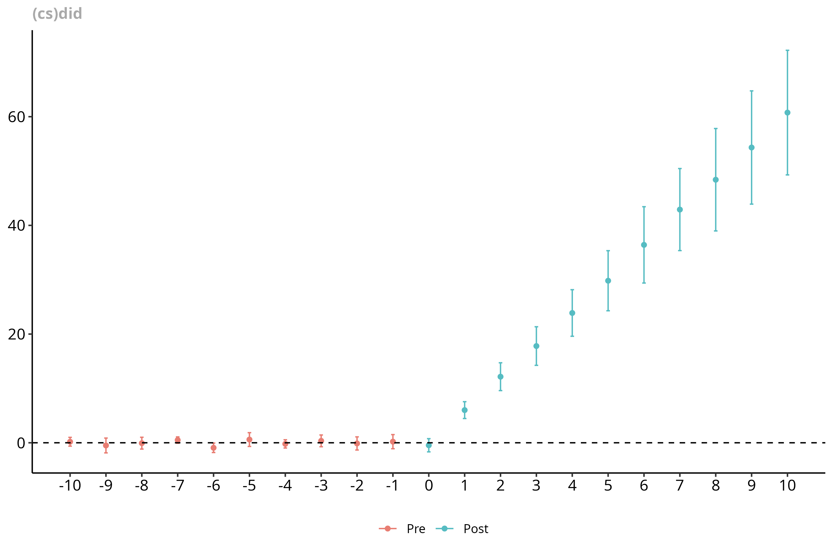
A final cherry on the top for did is that it provides a full set of methods
for post-estimation tidying and visualization. (Looking at you,
DIDmultiplegt.) Here’s a quick example using the latter, using the
ggdid() function
to produce an event-study plot.
ggdid(cs21_es, title = "(cs)did")