csdid
Table of contents
Notes
- Based on: Callaway and Sant’Anna 2021
- Program version (if available): v1.72
- Last checked: Nov 2024
Installation
ssc install csdid, replace
Take a look at the help file:
help csdid
Test the command
Please make sure that you generate the data using the script given here
For csdid we need the gvar variable which equals the first_treat value for the treated, and 0 for the not treated:
gen gvar = first_treat
recode gvar (. = 0)
Let’s try the basic csdid command:
csdid Y, ivar(id) time(t) gvar(gvar) notyet
And a very very long output will show up on the screen (combination explosion)! We can recover an event study with 10 leads and 10 lags as a post-estimation option:
estat event, window(-10 10) estore(cs)
which will show this output:
ATT by Periods Before and After treatment
Event Study:Dynamic effects
------------------------------------------------------------------------------
             | Coefficient  Std. err.      z    P>|z|     [95% conf. interval]
-------------+----------------------------------------------------------------
        Tm10 |   .3917418   .3493034     1.12   0.262    -.2928803    1.076364
         Tm9 |  -.0720548   .2991634    -0.24   0.810    -.6584043    .5142947
         Tm8 |   .0197712   .3119967     0.06   0.949    -.5917311    .6312735
         Tm7 |  -.2900224    .346774    -0.84   0.403    -.9696869    .3896422
         Tm6 |  -.1089479   .3190294    -0.34   0.733     -.734234    .5163383
         Tm5 |    .092667   .3352292     0.28   0.782    -.5643702    .7497042
         Tm4 |   .2572878   .3222909     0.80   0.425    -.3743907    .8889663
         Tm3 |   .0639963   .4214074     0.15   0.879    -.7619471    .8899396
         Tm2 |   .1944381   .3707239     0.52   0.600    -.5321673    .9210435
         Tm1 |  -.1308918   .4307277    -0.30   0.761    -.9751027     .713319
         Tp0 |  -.0608394   .3220462    -0.19   0.850    -.6920383    .5703595
         Tp1 |    8.49767   .3964781    21.43   0.000     7.720587    9.274753
         Tp2 |   17.64773   .4650298    37.95   0.000     16.73629    18.55917
         Tp3 |    25.9377   .5978201    43.39   0.000     24.76599     27.1094
         Tp4 |   34.62362   .9250424    37.43   0.000     32.81057    36.43667
         Tp5 |   42.85682   1.223002    35.04   0.000     40.45978    45.25386
         Tp6 |   51.93103   1.529193    33.96   0.000     48.93387    54.92819
         Tp7 |   60.13327   1.804358    33.33   0.000     56.59679    63.66975
         Tp8 |   68.82446   1.982765    34.71   0.000     64.93831    72.71061
         Tp9 |   77.30792   2.264938    34.13   0.000     72.86872    81.74712
        Tp10 |   85.78878    2.61102    32.86   0.000     80.67128    90.90629
------------------------------------------------------------------------------
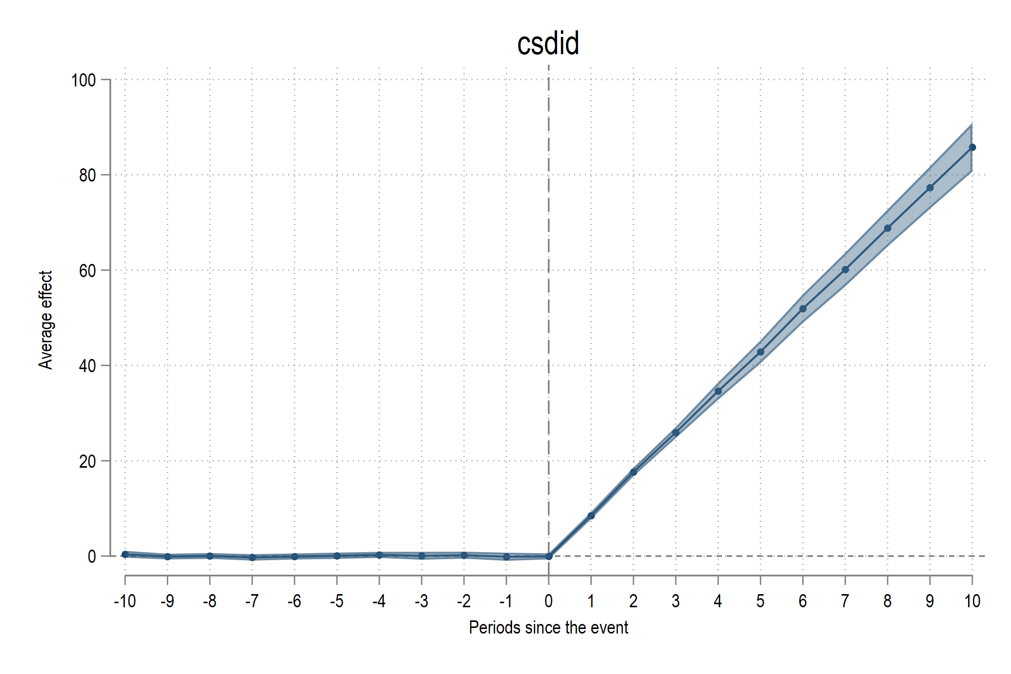
In order to plot the estimates we can use the event_plot (ssc install event_plot, replace) command as follows:
event_plot cs, default_look graph_opt(xtitle("Periods since the event") ytitle("Average effect") ///
	title("csdid") xlabel(-10(1)10)) stub_lag(Tp#) stub_lead(Tm#) together
And we get this figure: