csdid
Table of contents
Notes
- Based on: Callaway and Sant’Anna 2021
-
Program version (if available): v1.72
- Last checked: 7 Jul 2026
Installation
ssc install csdid, replace
Take a look at the help file:
help csdid
Test the command
Please make sure that you generate the shared setup data using the setup block given here
For csdid we need the gvar variable which equals the first_treat value for the treated, and 0 for the not treated:
gen gvar = first_treat
recode gvar (. = 0)
Let’s try the basic csdid command:
csdid Y, ivar(id) time(t) gvar(gvar) notyet
And a very very long output will show up on the screen (combination explosion)! We can recover an event study with 10 leads and 10 lags as a post-estimation option:
... output truncated for readability (many cohort-by-time ATT lines omitted) ...
Difference-in-difference with Multiple Time Periods

                                                         Number of obs = 1,800
Outcome model  : regression adjustment
Treatment model: none
------------------------------------------------------------------------------
             | Coefficient  Std. err.      z    P>|z|     [95% conf. interval]
-------------+----------------------------------------------------------------
g24          |
     t_21_22 |    .160638    .799291     0.20   0.841    -1.405944     1.72722
     t_23_25 |   9.664644     .60479    15.98   0.000     8.479278    10.85001
     t_23_30 |    60.1293   .4613613   130.33   0.000     59.22504    61.03355
-------------+----------------------------------------------------------------
g34          |
     t_33_35 |   7.874027   .7183369    10.96   0.000     6.466112    9.281941
     t_33_40 |   48.15233   .6323252    76.15   0.000       46.913    49.39167
     t_33_60 |   209.0268   .6309236   331.30   0.000     207.7902    210.2634
-------------+----------------------------------------------------------------
g38          |
     t_37_39 |   8.431514    .442824    19.04   0.000     7.563595    9.299433
     t_37_49 |    78.7768   .4526795   174.02   0.000     77.88957    79.66404
     t_37_60 |   155.3342   .6263662   247.99   0.000     154.1065    156.5618
-------------+----------------------------------------------------------------
g56          |
     t_55_57 |   7.908278   .8042398     9.83   0.000     6.331997    9.484559
     t_55_58 |   17.82876   .7229703    24.66   0.000     16.41177    19.24576
     t_55_60 |   35.58904   1.185714    30.01   0.000     33.26509      37.913
------------------------------------------------------------------------------
Control: Not yet Treated

See Callaway and Sant'Anna (2021) for details
which will show this output:
ATT by Periods Before and After treatment
Event Study:Dynamic effects
------------------------------------------------------------------------------
             | Coefficient  Std. err.      z    P>|z|     [95% conf. interval]
-------------+----------------------------------------------------------------
        Tm10 |   .3917418   .3493034     1.12   0.262    -.2928803    1.076364
         Tm9 |  -.0720548   .2991634    -0.24   0.810    -.6584043    .5142947
         Tm8 |   .0197712   .3119967     0.06   0.949    -.5917311    .6312735
         Tm7 |  -.2900224    .346774    -0.84   0.403    -.9696869    .3896422
         Tm6 |  -.1089479   .3190294    -0.34   0.733     -.734234    .5163383
         Tm5 |    .092667   .3352292     0.28   0.782    -.5643702    .7497042
         Tm4 |   .2572878   .3222909     0.80   0.425    -.3743907    .8889663
         Tm3 |   .0639963   .4214074     0.15   0.879    -.7619471    .8899396
         Tm2 |   .1944381   .3707239     0.52   0.600    -.5321673    .9210435
         Tm1 |  -.1308918   .4307277    -0.30   0.761    -.9751027     .713319
         Tp0 |  -.0608394   .3220462    -0.19   0.850    -.6920383    .5703595
         Tp1 |    8.49767   .3964781    21.43   0.000     7.720587    9.274753
         Tp2 |   17.64773   .4650298    37.95   0.000     16.73629    18.55917
         Tp3 |    25.9377   .5978201    43.39   0.000     24.76599     27.1094
         Tp4 |   34.62362   .9250424    37.43   0.000     32.81057    36.43667
         Tp5 |   42.85682   1.223002    35.04   0.000     40.45978    45.25386
         Tp6 |   51.93103   1.529193    33.96   0.000     48.93387    54.92819
         Tp7 |   60.13327   1.804358    33.33   0.000     56.59679    63.66975
         Tp8 |   68.82446   1.982765    34.71   0.000     64.93831    72.71061
         Tp9 |   77.30792   2.264938    34.13   0.000     72.86872    81.74712
        Tp10 |   85.78878    2.61102    32.86   0.000     80.67128    90.90629
------------------------------------------------------------------------------
Command results
The full csdid output is very long because it reports group-time effects for each cohort. Additional outputs show a few checkpoints:
| Checkpoint | Estimate | Notes |
|---|---|---|
| Observations | 1,800 | Full sample in the run |
g24, first reported post effect (t_23_25) |
9.6646 | Large and significant |
g24, later post effect (t_23_30) |
60.1293 | Dynamic effects accumulate |
g24, pre period (t_21_22) |
0.1606 | Close to zero |
These checkpoints line up with the simulated design where treatment effects grow with event time.
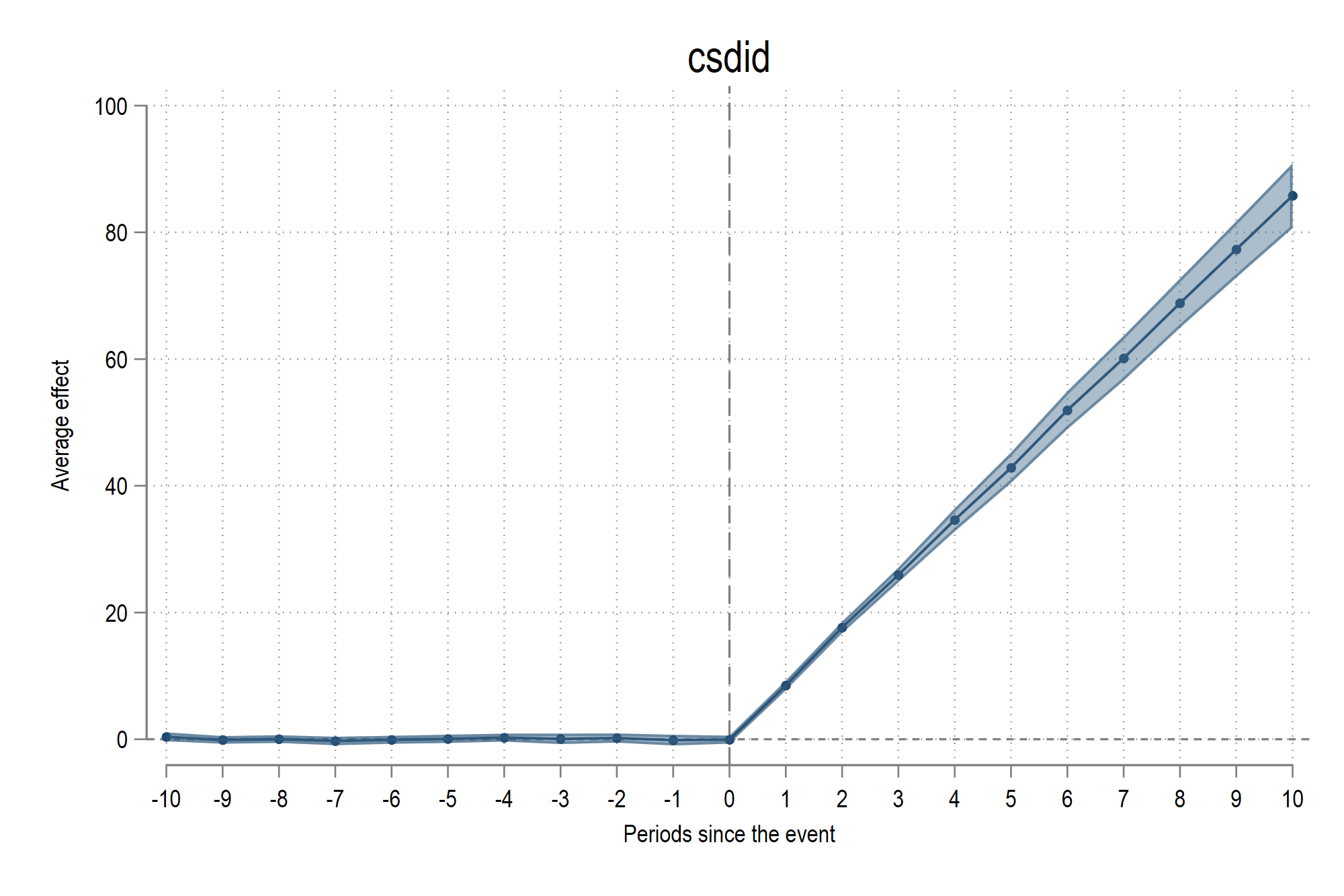
In order to plot the estimates we can use the event_plot (ssc install event_plot, replace) command as follows:
event_plot cs, default_look graph_opt(xtitle("Periods since the event") ytitle("Average effect") ///
	title("csdid") xlabel(-10(1)10)) stub_lag(Tp#) stub_lead(Tm#) together
And we get this figure: