did2s
Table of contents
Notes
- Based on: Gardner (2022). Two-stage Difference-in-Differences.
-
Program version (if available): 0.5
-
Last checked: 7 Jul 2026
- Additional info: See blog post for more details.
Installation
ssc install did2s, replace
Take a look at the help file:
help did2s
Test the command
Let’s try the basic did2s command:
did2s Y, first_stage(id t) second_stage(F_* L_*) treatment(D) cluster(id)
which will show this output:
(0 observations deleted)
                                     (Std. err. adjusted for clustering on id)
------------------------------------------------------------------------------
             | Coefficient  Std. err.      z    P>|z|     [95% conf. interval]
-------------+----------------------------------------------------------------
         F_2 |   .2253244   .2283664     0.99   0.324    -.2222655    .6729143
         F_3 |    .128698   .2330633     0.55   0.581    -.3280976    .5854936
         F_4 |  -.1034735   .2192386    -0.47   0.637    -.5331733    .3262262
         F_5 |   .0552204   .1902649     0.29   0.772     -.317692    .4281327
         F_6 |  -.1979187   .2035536    -0.97   0.331    -.5968765     .201039
         F_7 |  -.1802993   .2227204    -0.81   0.418    -.6168234    .2562247
         F_8 |   .0756883    .171078     0.44   0.658    -.2596184     .410995
         F_9 |   .0365711   .2131956     0.17   0.864    -.3812847    .4544268
        F_10 |   .0605167   .1874084     0.32   0.747    -.3067969    .4278304
         L_0 |   .0791996   .2777527     0.29   0.776    -.4651857     .623585
         L_1 |   8.619413   .3308806    26.05   0.000     7.970899    9.267927
         L_2 |   17.63192   .4282092    41.18   0.000     16.79265     18.4712
         L_3 |   26.00454   .6607589    39.36   0.000     24.70947     27.2996
         L_4 |   34.69155   .9381719    36.98   0.000     32.85277    36.53034
         L_5 |   42.57469   1.320413    32.24   0.000     39.98673    45.16266
         L_6 |    51.8403   1.579741    32.82   0.000     48.74407    54.93654
         L_7 |   59.97723   1.915125    31.32   0.000     56.22366    63.73081
         L_8 |   68.85919   2.106983    32.68   0.000     64.72958     72.9888
         L_9 |   77.24698   2.324845    33.23   0.000     72.69037    81.80359
        L_10 |   85.82518   2.650682    32.38   0.000     80.62994    91.02042
------------------------------------------------------------------------------
Command results
Additional diagnostics show key values:
| Metric | Value |
|---|---|
| Event-study sample | 1,800 |
On-impact effect (L_0) |
0.0792 |
First post period (L_1) |
8.6194 |
Tenth post period (L_10) |
85.8252 |
Example lead (F_2) |
0.2253 |
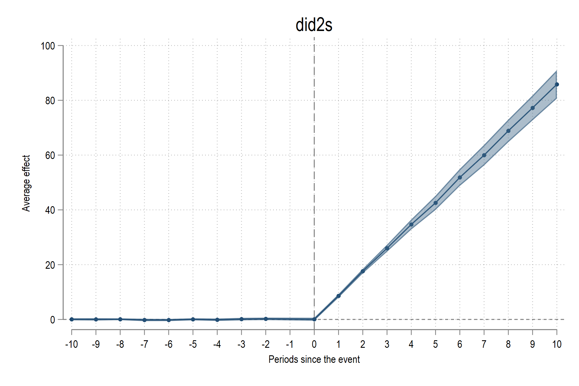
The shape mirrors other estimators in this dataset: near-zero pre period, then increasing post effects.
In order to plot the estimates we can use the event_plot (ssc install event_plot, replace) command as follows:
	event_plot, default_look graph_opt(xtitle("Periods since the event") ytitle("Average effect") xlabel(-10(1)10) ///
		title("did2s")) stub_lag(L_#) stub_lead(F_#) together
And we get this figure: